Simulation Overview
The behavior of a trebuchet cannot be described with a single set of equations. During different parts of its launch, a trebuchet is subject to different constraints. The obvious change in constraints during the launch happens when the projectile is released from the sling and is no longer attached to the trebuchet. There is another, less obvious, change that also happens during the launch. At the beginning of the launch, the projectile moves along the ground. It has no vertical component to its movement. At some point, the constraints change and the projectile leaves the ground.
In this simulation, the trebuchet launch is divided into three stages, each with its own set of equations. There is a specific condition that is monitored at each stage. When that condition is met the simulation moves onto the next stage.
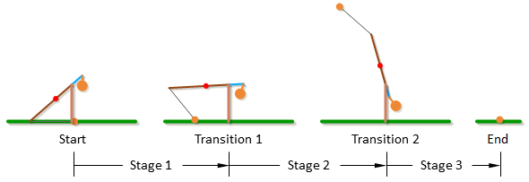
In stage 1 of the trebuchet simulation, the projectile is in contact with the ground and can only move in a direction parallel with the ground. During stage 1 the program keeps track of the force that the ground applies to the projectile to keep it moving along a horizontal path. At the beginning of the launch gravity wants to pull the projectile into the ground and the ground must push up on the projectile to keep it moving horizontally. After a certain point however, the sling pulls up on the projectile with a larger force than gravity pulls it down and the projectile transitions from pushing into the ground to pulling away from the ground. At this point, the ground would have to pull down on the projectile to keep it moving horizontally. When this transition from pushing to pulling occurs, the simulation is triggered to transition from stage 1 to stage 2.
In stage 2, the projectile at the end of the sling is free to move, unconstrained by the ground. In stage 2 the program keeps track of the angle of the velocity vector of the projectile relative to the ground, and when the angle of the velocity vector gets within a certain tolerance of the user specified release angle, the simulation is triggered to transition from stage 2 to stage 3. This transition is the release point.
In stage 3, the projectile is completely independent of the trebuchet. In stage 3 the program keeps track of the height of the projectile relative to ground. When the height becomes negative, that is the projectile goes below the ground, the simulation ends.
Example Problem
This section does not directly have anything to do with a trebuchet; rather it is an example problem that is used to explain generally the method that I use to make a simulation of a system. If you do not have much experience with simulation, studying this simple example problem will make the trebuchet equations easier to understand.
Developing Equations of Motion
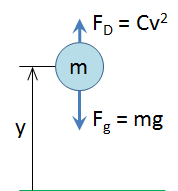
For the example problem we will consider a body in free fall. The first thing we need to do is develop the equations of motion for this system. This is a one-dimensional single body system, so there is only one degree of freedom and thus only one equation of motion.
F
g= gravitational forceF
D= force of dragm = mass of the body
g = gravitational constant
C = a constant that depends on the density of the air, the coefficient of drag of the body, and the reference area of the body
v = the velocity of the body
y = height of the body from the ground
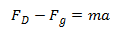
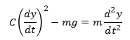
In order to find the equation of motion for this system we will use Newton’s second law: the sum of the forces acting on a body is equal the mass times the acceleration of that body.

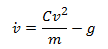
The forces acting on a body in free fall are gravity and the force of drag, so we get,
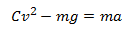
Plugging in the equations for gravity and drag results in,
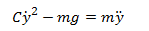
Next we will rewrite the equation in terms of y, where y is the height of the body from the ground. Velocity, v, is the first time-derivative of y, and acceleration, a, is the second time-derivative of y.
I prefer to use dot notation.
We will rewrite this equation in terms of ÿ.
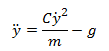
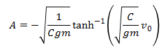
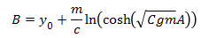
This is the equation of motion for this system. What we really want, however, is an expression for y as a function of time. Since the equation of motion we derived is relatively simple, it is not too difficult to solve it analytically to get y as a function of time. We will not go into the theory behind solving differential equations analytically, but the result of solving our equation of motion for y would be
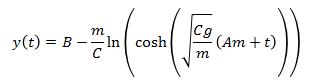
If we were only interested in this problem we could stop here, but we want to solve this problem in a way that is applicable to the trebuchet simulation. It is apparent from this example that the analytical solution for even a simple equation of motion can be fairly complex. For systems with much more complex equations of motion, like the equations of motion for a trebuchet, finding an analytical solution is nearly impossible, so we resort to solving the equation of motion using numerical methods.
Numerical Methods
What we get from a numerical method is different from what we get from an analytical solution. With an analytical solution the result is an expression for the variable(s) of interest as a function of time, and any arbitrary value for time can be plugged into the function to get the value of the variable(s) at that particular time. Using a numerical method will not give us a time function for the variable(s) of interest. With a numerical method we start at a known value for the variable(s), and then calculate what the variable(s) will be after a little bit of time has elapsed. Then we take the new value(s) and calculate what the variable(s) will be after a little more time has elapsed. We keep repeating this to see what the variable(s) do over time. Another thing that is different is that a numerical solution is only an approximation. It can be a very good approximation if it is done right, but it is an approximation none the less, so it is important to evaluate if the error is small enough.
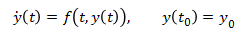
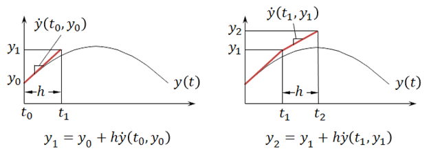
The numerical method we will use for this example is the Euler method. The Euler method assumes you have a function that describes the first derivative of a variable with respect to time, and that you know the initial condition of that variable. The initial condition is what the value of the variable is at time t = 0.
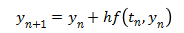
The way the Euler method works is that it takes the current value of y and uses the equation for the time derivative of y to approximate what the value of y will be after some time interval, h.
This equation is easier to visualize with a chart. Note that when using numerical methods y(t) is
not usually known. It is just shown on the chart below for visualization purposes.
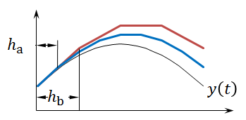
Notice the Euler approximation of y does not line up exactly with the actual value of y. This is because the Euler method is just an approximation. If the time interval h is made smaller, then the approximation can be improved. In the chart below the time interval, h, for the blue line is half of that of the red line, and it comes closer to the true curve for y(t).
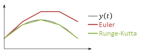
Using a smaller time interval, h, is not the only way to get a more accurate approximation. Another way to get a more accurate result is to use a higher order method. For example, the chart below compares the Euler method to the fourth-order Runge-Kutta method. The same time interval, h, is used for both methods. The fourth-order Runge-Kutta method is much more accurate given the same time interval.
The trebuchet simulation uses the fourth and fifth-order Runge-Kutta methods. However, the higher order methods are more complicated, so for the example problem we will use the Euler method since it is more concise, and the same procedure can be applied to the other methods. The equations for the fourth and fifth-order Runge-Kutta methods are given in the Runge-Kutta section.
Solving the Example Problem Using Numerical Methods
If we want to apply the Euler method to our example problem, we first need to get the equation of motion into the correct form. Remember that the Euler method assumes that we have an expression for the first order derivative of our variable(s) of interest. Our equation of motion, however, is a second order differential equation.
Somehow we need to get first order differential equation(s) from the equation of motion. We will do this by defining a new variable, v (velocity of the body).

If we plug v into our equation of motion we get
Now we have two variables, y and v, and we have expressions for the first order derivative of each variable.

Now we can use the Euler method to solve these equations numerically. Using the Euler method does not give us a general solution to the equations. It is used to find the solution for a particular case, so to continue the example we have to assign values to all the system parameters, and solve the problem for that specific case. We will use the following values for the system parameters.
g (gravitational constant) = 9.8 m/s² (in the negative y direction)
m (mass of body) = 1 kg
C (drag constant) = 0.015 kg/m
y₀ (initial height of body) = 10 m
v₀ (initial velocity of body) = 3 m/s (in the positive y direction)
h (time interval) = 0.1 s
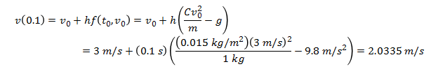
Now that we have given values to all the parameters, we can use the Euler method to find the position of the body after 0.1 seconds.

Now we have the approximate values for the height of the ball and the velocity of the ball after 0.1 seconds, and we can use that result to find the values after 0.2 seconds.


We can repeat this process for as much time as we are interested in. For this example we will follow the body until it reaches the ground. To be concise, we will not show the full equations for every step, rather the results will be summarized in the following table.
| Step | t (s) | y (m) | v (m/s) |
|---|---|---|---|
| 0 | 0.0 | 10.0000 | 3.0000 |
| 1 | 0.1 | 10.3000 | 2.0335 |
| 2 | 0.2 | 10.5034 | 1.0597 |
| 3 | 0.3 | 10.6093 | 0.0814 |
| 4 | 0.4 | 10.6175 | -0.8986 |
| 5 | 0.5 | 10.5276 | -1.8774 |
| 6 | 0.6 | 10.3399 | -2.8521 |
| 7 | 0.7 | 10.0546 | -3.8199 |
| 8 | 0.8 | 9.6727 | -4.7780 |
| 9 | 0.9 | 9.1949 | -5.7238 |
| 10 | 1.0 | 8.6225 | -6.6546 |
| 11 | 1.1 | 7.9570 | -7.5682 |
| 12 | 1.2 | 7.2002 | -8.4623 |
| 13 | 1.3 | 6.3540 | -9.3349 |
| 14 | 1.4 | 5.4205 | -10.1842 |
| 15 | 1.5 | 4.4021 | -11.0086 |
| 16 | 1.6 | 3.3012 | -11.8068 |
| 17 | 1.7 | 2.1205 | -12.5777 |
| 18 | 1.8 | 0.8628 | -13.3204 |
| 19 | 1.9 | -0.4693 | -14.0343 |
We can see that at step 19 the value for y went negative which means the body hit the ground sometime between 1.8 and 1.9 seconds. The results of this problem summarized in the table are plotted in the graph below.
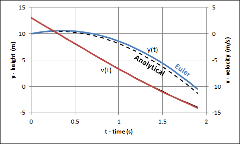
As mentioned before this is only an approximation of the results. Since we also have the analytical solution to this problem we can compare the results that we got from using the Euler method to the exact values from the analytical solution. The dotted line shows the analytical solution.
This simple example should have demonstrated the essentials of what is needed to understand what is going on in the trebuchet simulation. First the equations of motion are derived. They are then then reduced to first order differential equations and then solved using a numerical method like the Euler or Runge-Kutta method.
This example problem should have helped prepared you for the Equations of Motion and Runge-Kutta sections.
Equations of Motion
This section gives the equations for a trebuchet. I would suggest working through this Example Problem to understand the basics of how the equations work before trying work through this section.
The equations of motion for the trebuchet are a set of second order differential equations. The numerical methods used in the simulation only work with first order differential equations, so the derivatives of the motion variables were also renamed as separate variables which allowed the equations of motion to be rewritten as a set of first order differential equations. Those first order differential equations are presented in this section. There are a different set of equations for each stage of the trebuchet as described in the Simulation Overview.
The equations of motion for the trebuchet were derived using a program called Autolev. See the Autolev section to see the code that was actually used to develop the equations of motion.
Stage 1:
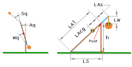
In stage 1 the motion variables are Aq, Wq, and Sq, and the constant lengths are LAl, LAs, LAcg, LW, LS, and h.
The time derivative of a variable is denoted by appending it with a '. For example Aq' means dAq/dt, and Sq'' means d²Sq/dt².
Additional constants not shown above are:
Grav = Gravitational Acceleration
mA = Mass of Arm
mW = Mass of Weight
mP = Mass of Projectile
IA3 = Inertia of Arm
IW3 = Inertia of Weight
The equations of motion for stage 1 are:
(-mP*LAl^2*(-1+2*SIN(Aq)*COS(Sq)/SIN(Aq+Sq)) + IA3 + IW3 + mA*LAcg^2 +
		mP*LAl^2*SIN(Aq)^2/SIN(Aq+Sq)^2 + mW*(LAs^2+LW^2+2*LAs*LW*COS(Wq)))*
Aq'' + (IW3 + LW*mW*(LW+LAs*COS(Wq)))*Wq''
= Grav*LAcg*mA*SIN(Aq) +
		LAl*LS*mP*(SIN(Sq)*(Aq'+Sq')^2+COS(Sq)*(COS(Aq+Sq)*Sq'*(Sq'+2*Aq')/SIN(Aq+Sq)+(COS(Aq+Sq)/SIN(Aq+Sq)+LAl*COS(Aq)/(LS*SIN(Aq+Sq)))*Aq'^2))
		+
		LAl*mP*SIN(Aq)*(LAl*SIN(Sq)*Aq'^2-LS*(COS(Aq+Sq)*Sq'*(Sq'+2*Aq')/SIN(Aq+Sq)+(COS(Aq+Sq)/SIN(Aq+Sq)+LAl*COS(Aq)/(LS*SIN(Aq+Sq)))*Aq'^2))/SIN(Aq+Sq)
		- Grav*mW*(LAs*SIN(Aq)+LW*SIN(Aq+Wq)) - LAs*LW*mW*SIN(Wq)*(Aq'^2-(Aq'+Wq')^2)
(IW3 + LW*mW*(LW+LAs*COS(Wq)))*Aq''
+ (IW3 + mW*LW^2)*Wq''
= -LW*mW*(Grav*SIN(Aq+Wq)+LAs*SIN(Wq)*Aq'^2)
Note that in stage 1, when the ball is on the ground, the trebuchet only has two degrees of freedom, which is why there are only two equations of motion. However there were three variables to begin with. This works because Sq’ becomes a dependent variable defined by the expression,
Sq'= -(LAl*SIN(Aq)+LS*SIN(Aq+Sq))*Aq'/(LS*SIN(Aq+Sq))
and Sq’’ becomes,
Sq''= -COS(Aq+Sq)*Sq'*(Sq'+2*Aq')/SIN(Aq+Sq) -
(COS(Aq+Sq)/SIN(Aq+Sq)+LAl*COS(Aq)/(LS*SIN(Aq+Sq)))*Aq'^2 -
(LAl*SIN(Aq)+LS*SIN(Aq+Sq))*Aq''/(LS*SIN(Aq+Sq))
As is discussed in the Example Problem, complex differential equations like this are practically impossible to solve analytically. As a result, numerical methods must be used to approximate an answer. These methods require that the equations of motion to be reduced to first order differential equations. In order to accomplish this, we will define three new variables Aw, Ww, and Sw which are the the time derivatives of Aq, Wq, and Sq.
Aw = Aq'
Ww = Wq'
Sw = Sq'
Substituting Aw, Ww, and Sw in to the equations of motion gives,
(-mP*LAl^2*(-1+2*SIN(Aq)*COS(Sq)/SIN(Aq+Sq)) + IA3 + IW3 + mA*LAcg^2 +
		mP*LAl^2*SIN(Aq)^2/SIN(Aq+Sq)^2 + mW*(LAs^2+LW^2+2*LAs*LW*COS(Wq)))*
Aw' + (IW3 + LW*mW*(LW+LAs*COS(Wq)))*Ww'
= Grav*LAcg*mA*SIN(Aq) +
		LAl*LS*mP*(SIN(Sq)*(Aw+Sw)^2+COS(Sq)*(COS(Aq+Sq)*Sw*(Sw+2*Aw)/SIN(Aq+Sq)+(COS(Aq+Sq)/SIN(Aq+Sq)+LAl*COS(Aq)/(LS*SIN(Aq+Sq)))*Aw^2))
		+
		LAl*mP*SIN(Aq)*(LAl*SIN(Sq)*Aw^2-LS*(COS(Aq+Sq)*Sw*(Sw+2*Aw)/SIN(Aq+Sq)+(COS(Aq+Sq)/SIN(Aq+Sq)+LAl*COS(Aq)/(LS*SIN(Aq+Sq)))*Aw^2))/SIN(Aq+Sq)
		- Grav*mW*(LAs*SIN(Aq)+LW*SIN(Aq+Wq)) - LAs*LW*mW*SIN(Wq)*(Aw^2-(Aw+Ww)^2)
(IW3 + LW*mW*(LW+LAs*COS(Wq)))*Aw'
+ (IW3 + mW*LW^2)*Ww'
= -LW*mW*(Grav*SIN(Aq+Wq)+LAs*SIN(Wq)*Aw^2)
which are now first order differntial equations. As discussed in the Example Problem, we need to get the equations into the form,
y'(t) = f(t, y(t))
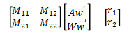
Separating Aw’ and Ww’ into separate expressions will require a little linear algebra. So, first
we will write the equations of motion in matrix form.
where,
M11= -mP*LAl^2*(-1+2*SIN(Aq)*COS(Sq)/SIN(Aq+Sq)) + IA3 + IW3 + mA*LAcg^2 +
mP*LAl^2*SIN(Aq)^2/SIN(Aq+Sq)^2 + mW*(LAs^2+LW^2+2*LAs*LW*COS(Wq))
M12= IW3 + LW*mW*(LW+LAs*COS(Wq))
M21= IW3 + LW*mW*(LW+LAs*COS(Wq))
M22= IW3 + mW*LW^2
r1= Grav*LAcg*mA*SIN(Aq) +
LAl*LS*mP*(SIN(Sq)*(Aw+Sw)^2+COS(Sq)*(COS(Aq+Sq)*Sw*(Sw+2*Aw)/SIN(Aq+Sq)+(COS(Aq+Sq)/SIN(Aq+Sq)+LAl*COS(Aq)/(LS*SIN(Aq+Sq)))*Aw^2))
+
LAl*mP*SIN(Aq)*(LAl*SIN(Sq)*Aw^2-LS*(COS(Aq+Sq)*Sw*(Sw+2*Aw)/SIN(Aq+Sq)+(COS(Aq+Sq)/SIN(Aq+Sq)+LAl*COS(Aq)/(LS*SIN(Aq+Sq)))*Aw^2))/SIN(Aq+Sq)
- Grav*mW*(LAs*SIN(Aq)+LW*SIN(Aq+Wq)) - LAs*LW*mW*SIN(Wq)*(Aw^2-(Aw+Ww)^2)
r2= -LW*mW*(Grav*SIN(Aq+Wq)+LAs*SIN(Wq)*Aw^2)
We can solve for Aw' and Ww' by multiplying both sides of the equation by the inverse of matrix M.
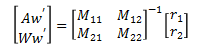
which give the result,
Aw'= (r1*M22-r2*M12)/(M11*M22-M12*M21)
Ww'= -(r1*M21-r2*M11)/(M11*M22-M12*M21)
In summary, the equations that are used by the simulation for stage 1 are,
Aq'= Aw
Wq'= Ww
Sq'= Sw
Aw'= (r1*M22-r2*M12)/(M11*M22-M12*M21)
Ww'= -(r1*M21-r2*M11)/(M11*M22-M12*M21)
Sw'= -COS(Aq+Sq)*Sq'*(Sq'+2*Aq')/SIN(Aq+Sq) -
(COS(Aq+Sq)/SIN(Aq+Sq)+LAl*COS(Aq)/(LS*SIN(Aq+Sq)))*Aq'^2 -
(LAl*SIN(Aq)+LS*SIN(Aq+Sq))*Aq''/(LS*SIN(Aq+Sq))
As described in the Example Problem, these first order differential equations are solved using the numerical methods described in the Runge-Kutta section, and the results are values for the angles (Aq, Wq, Sq) and their derivatives (Aw, Ww, Sw) over time. These angles can be converted into X and Y coordinates using the expressions found in the Angles to XY Coordinates section.
Stage 2:
In stage 2 the parameters are the same as in stage 1. The equations of motion for stage 2 are:
(IA3 + IW3 + mA*LAcg^2 + mP*(LAl^2+LS^2+2*LAl*LS*COS(Sq)) +
		mW*(LAs^2+LW^2+2*LAs*LW*COS(Wq)))*
Aq'' + (IW3 + LW*mW*(LW+LAs*COS(Wq)))*Wq'' + (LS*mP*(LS+LAl*COS(Sq)))*Sq''
= Grav*LAcg*mA*SIN(Aq) + Grav*mP*(LAl*SIN(Aq)+LS*SIN(Aq+Sq)) -
		Grav*mW*(LAs*SIN(Aq)+LW*SIN(Aq+Wq)) - LAl*LS*mP*SIN(Sq)*(Aq'^2-(Aq'+Sq')^2) -
		LAs*LW*mW*SIN(Wq)*(Aq'^2-(Aq'+Wq')^2)
(IW3 + LW*mW*(LW+LAs*COS(Wq)))*Aq''
+ (IW3 + mW*LW^2)*Wq''
= -LW*mW*(Grav*SIN(Aq+Wq)+LAs*SIN(Wq)*Aq'^2)
(LS*mP*(LS+LAl*COS(Sq)))*Aq''
+ (mP*LS^2)*Sq''
= LS*mP*(Grav*SIN(Aq+Sq)-LAl*SIN(Sq)*Aq'^2)
Note that in stage 2, there are three degrees of freedom, so there are now three equations of motion. As in stage 1 we will turn the equations of motion onto first order differential equations by using the time derivatives of Aq, Wq, and Sq, which we will call Aw, Ww, and Sw, and substituting them into the equations of motion.
(IA3 + IW3 + mA*LAcg^2 + mP*(LAl^2+LS^2+2*LAl*LS*COS(Sq)) +
		mW*(LAs^2+LW^2+2*LAs*LW*COS(Wq)))*
Aw' + (IW3 + LW*mW*(LW+LAs*COS(Wq)))*Ww' + (LS*mP*(LS+LAl*COS(Sq)))*Sw'
= Grav*LAcg*mA*SIN(Aq) + Grav*mP*(LAl*SIN(Aq)+LS*SIN(Aq+Sq)) -
		Grav*mW*(LAs*SIN(Aq)+LW*SIN(Aq+Wq)) - LAl*LS*mP*SIN(Sq)*(Aw^2-(Aw+Sw)^2) -
		LAs*LW*mW*SIN(Wq)*(Aw^2-(Aw+Ww)^2)
(IW3 + LW*mW*(LW+LAs*COS(Wq)))*Aw'
+ (IW3 + mW*LW^2)*Ww'
= -LW*mW*(Grav*SIN(Aq+Wq)+LAs*SIN(Wq)*Aw^2)
(LS*mP*(LS+LAl*COS(Sq)))*Aw'
+ (mP*LS^2)*Sw'
= LS*mP*(Grav*SIN(Aq+Sq)-LAl*SIN(Sq)*Aw^2)
In order to separate Aw’, Ww’, and Sw’ into separate expressions we will first put the equations of motion into matrix form.
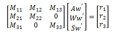
where,
M11= IA3 + IW3 + mA*LAcg^2 + mP*(LAl^2+LS^2+2*LAl*LS*COS(Sq)) +
mW*(LAs^2+LW^2+2*LAs*LW*COS(Wq))
M12= IW3 + LW*mW*(LW+LAs*COS(Wq))
M13= LS*mP*(LS+LAl*COS(Sq))
M21= IW3 + LW*mW*(LW+LAs*COS(Wq))
M22= IW3 + mW*LW^2
M31= LS*mP*(LS+LAl*COS(Sq))
M33= mP*LS^2
r1= Grav*LAcg*mA*SIN(Aq) + Grav*mP*(LAl*SIN(Aq)+LS*SIN(Aq+Sq)) -
Grav*mW*(LAs*SIN(Aq)+LW*SIN(Aq+Wq)) - LAl*LS*mP*SIN(Sq)*(Aw^2-(Aw+Sw)^2) -
LAs*LW*mW*SIN(Wq)*(Aw^2-(Aw+Ww)^2)
r2= -LW*mW*(Grav*SIN(Aq+Wq)+LAs*SIN(Wq)*Aw^2)
r3= LS*mP*(Grav*SIN(Aq+Sq)-LAl*SIN(Sq)*Aw^2)
Now, we can solve for Aw', Ww', and Sw’ by multiplying both sides of the equation by the inverse of matrix M.
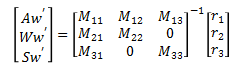
which gives the result used in the simulation,
Aq'= Aw
Wq'= Ww
Sq'= Sw
Aw'= -(r1*M22*M33-r2*M12*M33-r3*M13*M22)/(M13*M22*M31-M33*(M11*M22-M12*M21))
Ww'= (r1*M21*M33-r2*(M11*M33-M13*M31)-r3*M13*M21)/(M13*M22*M31-M33*(M11*M22-M12*M21))
Sw'= (r1*M22*M31-r2*M12*M31-r3*(M11*M22-M12*M21))/(M13*M22*M31-M33*(M11*M22-M12*M21))
As described in the Example Problem, these first order differential equations are solved using the numerical methods described in the Runge-Kutta section, and the results are values for the angles (Aq, Wq, Sq) and their derivatives (Aw, Ww, Sw) over time. These angles can be converted into X and Y coordinates using the expressions found in the Angles to XY Coordinates section.
Stage 3:
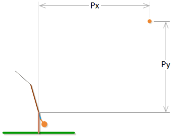
Stage 3 has a different set of parameters than stage 1 or 2. The motion variables are Px and Py. Note that in the simulation everything is measured relative to the pivot point.
The constant parameters in stage 3 are:
Grav = Gravitational Acceleration ρ = Density of Air
WS = Wind Speed
Aeff = Effective Area of the Projectile (= π*(Projectile Diameter/2)^2)
mP = Mass of Projectile
Cd = Drag Coefficient of Projectile
The drag coefficient is not actually a constant. It is related to the Reynolds number which is dependent on the velocity of the projectile relative to the air. For more information on how the drag coefficient is derived, see the Projectile Drag section.
The equations of motion for stage 3 are:
Px''= -(ρ*Cd*Aeff*(Px'-WS)*sqrt(Py'^2+(WS-Px')^2))/(2*mP)
Py''= -Grav - (ρ*Cd*Aeff*Py'*sqrt(Py'^2+(WS-Px')^2))/(2*mP)
In order to make the equations of motion into first order differential equations, we will define to new variables Pvx and Pvy which we will make equal to the time derivatives of Px and Py.
Pvx = Px'
Pvy = Py'
Substituting these into the equations of motion gives the expressions used in the simulation.
Px'= Pvx
Py'= Pvy
Pvx'= -(ρ*Cd*Aeff*(Pvx-WS)*sqrt(Pvy^2+(WS-Pvx)^2))/(2*mP)
Pvy'= -Grav - (ρ*Cd*Aeff*Pvy*sqrt(Pvy^2+(WS-Pvx)^2))/(2*mP)
As described in the Example Problem, these first order differential equations are solved using the numerical methods described in the Runge-Kutta section, and the results are values for the variables (Px, Py) and their derivatives (Pvx, Pvy) over time.
Angles to XY Coordinates
The equations of motion for the first two stages of the trebuchet given in the Equations of Motion section are used to find the angles (Aq, Wq, Sq) of the trebuchet over time. These angles can be used to find the Cartesian coordinates of the different parts of the trebuchet.
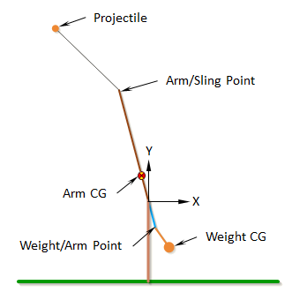
Weight CG:
X = LAs*SIN(Aq) + LW*SIN(Aq+Wq)
Y = -LAs*COS(Aq) - LW*COS(Aq+Wq)
Weight/Arm Point:
X = LAs*SIN(Aq)
Y = -LAs*COS(Aq)
Arm CG:
X = -LAcg*SIN(Aq)
Y = LAcg*COS(Aq)
Arm/Sling Point:
X = -LAl*SIN(Aq)
Y = LAl*COS(Aq)
Projectile:
X = -LAl*SIN(Aq) - LS*SIN(Aq+Sq)
Y = LAl*COS(Aq) + LS*COS(Aq+Sq)
Runge-Kutta
The Runge-Kutta methods are
a set of numerical methods for solving first order differential equations of the form,
They take the variable (y in the equation above) at a given time and use the known expression for
the derivative of the variable to approximate the value of the variable a small interval of time,
h, later in time. The simplest Runge-Kutta method is also known as the
Euler method which is what the
Example Problem used. It uses the
following expression to approximate what y will be after the time interval h.
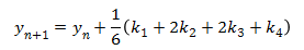
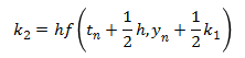
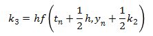
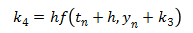
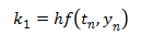
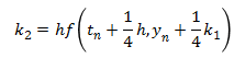
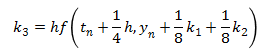
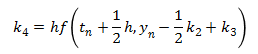
The Euler method is simple since it is only the first order Runge-Kutta, but it has poor accuracy. Much better accuracy can be obtained using the same step size, h, by using the following fourth order Runge-Kutta method. This fourth order Runge-Kutta method is probably the most commonly used Runge-Kutta method, as it it a good balance between accuracy and complexity.

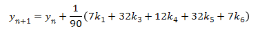
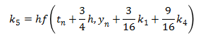
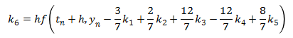
This next method is a version of the fifth order Runge-Kutta method. (There are several different versions of the higher order methods.) It is more accurate than the fourth order Runge-Kutta method, although it is also more complex.
The trebuchet simulation uses the fifth order Runge-Kutta method to solve the Equations of Motion. It also uses the fourth order Runge-Kutta method to check the accuracy of the solution. Any numerical method only gives an approximation of the actual answer, and its accuracy is dependent on the step size, h. The way the simulation determines it is using a small enough step size is that it compares the answers of the fourth and fifth order methods to make sure the answers agree within a specified tolerance of each other. If the answers are very close then the answer is considered to be a reasonable approximation, but if they aren’t close, the time step is made smaller until the answers do agree within the tolerance.
Projectile Drag
The force of drag (or air resistance) on an object is in the opposite direction of the velocity of that object relative to the air, and can be expressed by,
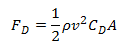
where
F
D= force of dragρ = density of air
v = velocity of the object relative to the air
A = cross-sectional area of the object
C
D= drag coefficient
In the original VirtualTrebuchet simulation the drag coefficient, CD, was assumed to
be a constant 0.47. This is a reasonable assumption over a certain velocity range.
In VirtualTrebuchet 2.0, the drag coefficient, CD, is not assumed to be a constant.
Instead the drag coefficient is continually recalculated during the simulation. It is derived by
first finding the Reynolds number of
the object at a particular time. The Reynolds number, Re, is non-dimensional number defined as,

where
v = velocity of the object relative to the air
D = diameter of the object
ν = the kinematic viscosity of the air
People have found the relationships between the Reynolds number and the drag coefficient for different shapes empirically. For the simulation, I used the charts in Figures 9.21 and 9.25 of the textbook, Fundamentals of Fluid Mechanics Fifth Edition to get the relationship between the Reynolds number and the drag coefficient for a smooth sphere. The following chart shows the approximate shape of this relationship.
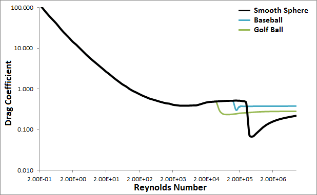
All the projectiles in the simulation are assumed to be smooth spheres except for the baseball and golf ball options. The simulation uses special curves for the baseball and golf ball as shown in the chart above. The data the simulation uses for the baseball and golf ball came from a paper by Rabindm D. Mehta and Jani Macari Pallis called Sports Ball Aerodynamics: Effects of Velocity, Spin and Surface Roughness (PDF).
Autolev
The equations of motion for the trebuchet were derived using a program called Autolev. The Autolev code that was used to derive the trebuchet equations will be included here with some minimal explanation. The figure below shows what the constants and variables in this code correspond to.
Stage 1 Autolev Code:
(1) % File: Trebuchet_Stage_1.al
(2) % Date: November 19, 2010
(3) % Author: Eric Olson
(4) % Problem: This is the first stage in a simulation of a trebuchet
(5) % shooting a projectile. In this stage the projectile
(6) % is in the sling, and is in contact with the ground.
(7) %--------------------------------------------------------------------
(8) % Default settings
Anything after a % symbol is just a comment.
(9) AutoEpsilon 1.0E-14 % Rounds off to nearest integer
(10) AutoZ OFF % Turn ON for large problems
(11) Digits 7 % Number of digits displayed for numbers
(12) BeepSound OFF
These are just program settings that can be ignored.
(13) %--------------------------------------------------------------------
(14) % Newtonian, bodies, frames, particles, points
(15) Newtonian N % Newtonian reference frame
The Newtonian reference frame is the base reference frame that everything else is based off of.
(16) Bodies A, W % Arm and Counterweight
A body has a local reference frame, a mass, a center of gravity, and inertia properties.
(17) Frames S % Sling
The sling is assumed to be massless, so it is defined as a frame instead of as a body.
(18) Particles P % Projectile
The projectile is assumed to be a point mass.
(19) %--------------------------------------------------------------------
(20) % Variables, constants, and specified
(21) Variables Aq', Wq', Sq' % Arm angle, Counterweight-arm angle, and Sling-arm
		angle
This defined the angles and their derivatives. The angles are the “motion variables”.
(22) Variables Fy % Normal Force of Projectile
This is the force that the ground exerts on the projectile in stage 1.
(23) Constants Grav % Local gravitational acceleration
(24) Constants LAs, LAl, LAcg % Length of long arm, length of short arm, distance from pivot to
		Arm CG.
(25) Constants LW, LS, h % Distance from arm end to Wo, length of sling, hight of pivot from
		the ground
(26) %--------------------------------------------------------------------
(27) % Motion variables for static/dynamic analysis
(28) Variables u3' % Motion variables; derivatives
(29) Aq' = u1
-> (30) Aq' = u1
The -> means that this line is program output.
(31) Wq' = u2
-> (32) Wq' = u2
(33) Sq' = u3
-> (34) Sq' = u3
This section defines the derivatives of the motion variables. This is done this way so that the equations for the trebuchet will be first order differential equations rather that second order differential equations. The numerical methods that are used to solve the final equations only work with first order differential equations. This is similar to what we did in the Example Problem.
(35) %--------------------------------------------------------------------
(36) % Quantities to be left explicit
(37) Zee_Not = [u1',u2',u3',Grav]
-> (38) Zee_Not = [u1', u2', u3', Grav]
With the initial settings that were set, this section does not do anything.
(39) %--------------------------------------------------------------------
(40) % Mass and inertia properties
(41) Mass A=mA, W=mW, P=mP
(42) Inertia A, IA1, IA2, IA3
-> (43) I_A_AO>> = IA1*A1>*A1> + IA2*A2>*A2> + IA3*A3>*A3>
(44) Inertia W, IW1, IW2, IW3
-> (45) I_W_WO>> = IW1*W1>*W1> + IW2*W2>*W2> + IW3*W3>*W3>
This section assigns mass and inertia to the bodies. The convention in Autolev is that 1 is x, 2 is y, and 3 is z. Anything with a > symbol is a vector, and anything with a >> is a tensor. A1> means the x direction of the local reference frame associated with body A.
(46) %--------------------------------------------------------------------
(47) % Geometry relating unit vectors
(48) Simprot(N, A, 3, Aq)
-> (49) N_A = [COS(Aq), -SIN(Aq), 0; SIN(Aq), COS(Aq), 0; 0, 0, 1]
(50) Simprot(A, W, 3, Wq)
-> (51) A_W = [COS(Wq), -SIN(Wq), 0; SIN(Wq), COS(Wq), 0; 0, 0, 1]
(52) Simprot(A, S, 3, Sq)
-> (53) A_S = [COS(Sq), -SIN(Sq), 0; SIN(Sq), COS(Sq), 0; 0, 0, 1]
This section defines the relationship between the different local reference frames and the Newtonian reference frame.
(54) %--------------------------------------------------------------------
(55) % Angular velocities
(56) W_A_N> = Aq'*N3>
-> (57) W_A_N> = u1*A3>
(58) W_W_A> = Wq'*A3>
-> (59) W_W_A> = u2*A3>
(60) W_S_A> = Sq'*A3>
-> (61) W_S_A> = u3*A3>
(62) %--------------------------------------------------------------------
(63) % Position vectors
(64) P_No_Ao> = LAcg*A2>
-> (65) P_No_Ao> = LAcg*A2>
(66) P_No_Wo> = -LAs*A2> - LW*W2>
-> (67) P_No_Wo> = -LAs*A2> - LW*W2>
(68) P_No_P> = LAl*A2> + LS*S2>
-> (69) P_No_P> = LAl*A2> + LS*S2>
This section defines the location of the different points of interest in the trebuchet. For example line 66 says the vector from the pivot (No) to the CG of the weight (Wo) is –LAs in the y component of the arm’s local coordinate system, and –LW in the y component of the weight’s local coordinate system.
(70) %--------------------------------------------------------------------
(71) % Velocities
(72) V_Ao_N> = Dt(P_No_Ao>,N)
-> (73) V_Ao_N> = -LAcg*u1*A1>
(74) V_Wo_N> = Dt(P_No_Wo>,N)
-> (75) V_Wo_N> = LAs*u1*A1> + LW*(u1+u2)*W1>
(76) V_P_N> = Dt(P_No_P>,N)
-> (77) V_P_N> = -LAl*u1*A1> - LS*(u1+u3)*S1>
The velocities vectors of the points of interest are defined as the time derivatives of the position vectors in reference to the Newtonian reference frame.
(78) Projectile_Vx = coef(express(V_P_N>,N),N1>)
-> (79) Projectile_Vx = -LAl*COS(Aq)*u1 - LS*COS(Aq+Sq)*(u1+u3)
(80) Projectile_Vy = coef(express(V_P_N>,N),N2>)
-> (81) Projectile_Vy = -LAl*SIN(Aq)*u1 - LS*SIN(Aq+Sq)*(u1+u3)
This finds the x and y component of the projectile velocity expressed in terms of the Newtonian reference frame.
(82) %--------------------------------------------------------------------
(83) % Motion constraints
(84) Auxiliary[1] = Projectile_Vy % P stays on ground
-> (85) Auxiliary[1] = Projectile_Vy
(86) Constrain(Auxiliary[u3])
-> (87) u3 = -(LAl*SIN(Aq)+LS*SIN(Aq+Sq))*u1/(LS*SIN(Aq+Sq))
-> (88) u3' = -COS(Aq+Sq)*u3*(u3+2*u1)/SIN(Aq+Sq) - (COS(Aq+Sq)/SIN(Aq+Sq)+LAl*
COS(Aq)/(LS*SIN(Aq+Sq)))*u1^2-(LAl*SIN(Aq)+LS*SIN(Aq+Sq))*u1'/(LS*SIN
(Aq+Sq))
This section constrains the y component of the projectiles velocity to be 0. This is what keeps the projectile moving along the ground in the first stage. This constraint eliminates one degree of freedom from the system and so one of the motion variables has to be rewritten in terms of the other motion variables. In this case u3 aka Sq’ is now given in terms of u1 and u2, and will not show up in the final equations.
(89) %Dependent[1] = Projectile_Vy % P stays on ground
(90) %Constrain(Dependent[u3])
(91) %--------------------------------------------------------------------
(92) % Angular accelerations
(93) ALF_A_N> = Dt(W_A_N>,N)
-> (94) ALF_A_N> = u1'*A3>
(95) ALF_W_N> = Dt(W_W_N>,N)
-> (96) ALF_W_N> = (u1'+u2')*W3>
(97) ALF_S_N> = Dt(W_S_N>,N)
-> (98) ALF_S_N> = (u1'+u3')*A3>
The angular accelerations are found by taking the time derivatives of the angular velocities.
(99) %--------------------------------------------------------------------
(100) % Accelerations
(101) A_Ao_N> = Dt(V_Ao_N>,N)
-> (102) A_Ao_N> = -LAcg*u1'*A1> - LAcg*u1^2*A2>
(103) A_Wo_N> = Dt(V_Wo_N>,N)
-> (104) A_Wo_N> = LAs*u1'*A1> + LAs*u1^2*A2> + LW*(u1'+u2')*W1> +
		LW*(u1+u2)^2
*W2>
(105) A_P_N> = Dt(V_P_N>,N)
-> (106) A_P_N> = -LAl*u1'*A1> - LAl*u1^2*A2> - LS*(u1'+u3')*S1> -
		LS*(u1+u3)^2
*S2>
The acceleration vectors of the points of interest are found by taking the derivative of the velocity vectors.
(107) %--------------------------------------------------------------------
(108) % Forces
(109) Force_P> = Fy*N2>
-> (110) Force_P> = Fy*N2>
This defines the force vector exerted on the projectile by the ground.
(111) Gravity(-Grav*N2>)
-> (112) FORCE_AO> = -Grav*mA*N2>
-> (113) FORCE_P> = (Fy-Grav*mP)*N2>
-> (114) FORCE_WO> = -Grav*mW*N2>
This defines the force vectors that gravity exerts on the bodies and point masses.
(115) %--------------------------------------------------------------------
(116) % Equations of motion
(117) Zero = Fr() + FrStar() % Find equations of motion
-> (118) Zero[1] = Grav*LAcg*mA*SIN(Aq) + (Grav*mP-Fy)*(LAl*SIN(Aq)+LS*SIN(Aq+
Sq)) - Grav*mW*(LAs*SIN(Aq)+LW*SIN(Aq+Wq)) - LAs*LW*mW*SIN(Wq)*(u1^2-(
u1+u2)^2) - LS*mP*(LAl*SIN(Sq)*u1^2-LAl*SIN(Sq)*(u1+u3)^2-LS*(COS(Aq+
Sq)*u3*(u3+2*u1)/SIN(Aq+Sq)+(COS(Aq+Sq)/SIN(Aq+Sq)+LAl*COS(Aq)/(LS*SIN
(Aq+Sq)))*u1^2)-LAl*COS(Sq)*(COS(Aq+Sq)*u3*(u3+2*u1)/SIN(Aq+Sq)+(COS(
Aq+Sq)/SIN(Aq+Sq)+LAl*COS(Aq)/(LS*SIN(Aq+Sq)))*u1^2)) - (IW3+LW*mW*(
LW+LAs*COS(Wq)))*u2' - (IA3+IW3+mA*LAcg^2+mW*(LAs^2+LW^2+2*LAs*LW*COS(
Wq))-mP*(LAl^2*SIN(Aq)*COS(Sq)/SIN(Aq+Sq)-LAl^2-LAl*LS*COS(Sq)-LS^2*(1
-(LAl*SIN(Aq)+LS*SIN(Aq+Sq))/(LS*SIN(Aq+Sq)))))*u1'
-> (119) Zero[2] = -Grav*LW*mW*SIN(Aq+Wq) - LAs*LW*mW*SIN(Wq)*u1^2 - (IW3+mW*
LW^2)*u2' - (IW3+LW*mW*(LW+LAs*COS(Wq)))*u1'
-> (120) Zero[3] = LS*(SIN(Aq+Sq)*(Grav*mP-Fy)+mP*(LS*(COS(Aq+Sq)*u3*(u3+2*u1)/
SIN(Aq+Sq)+(COS(Aq+Sq)/SIN(Aq+Sq)+LAl*COS(Aq)/(LS*SIN(Aq+Sq)))*u1^2)-
LAl*SIN(Sq)*u1^2-LAl*(COS(Sq)-SIN(Aq)/SIN(Aq+Sq))*u1'))
The trebuchet has been fully defined by all the previous sections. This section combines it all into the equations of motion of the trebuchet in stage 1. Notice that there are tree equations of motion but only two motion variables derivatives appear in these equations (u1 and u2). This is because u3 was turned into a dependent variable in line (86).
(121) Kane(Fy)
-> (122) Fy = mP*(Grav+(LS*(COS(Aq+Sq)*u3*(u3+2*u1)/SIN(Aq+Sq)+(COS(Aq+Sq)/SIN(
Aq+Sq)+LAl*COS(Aq)/(LS*SIN(Aq+Sq)))*u1^2)-LAl*SIN(Sq)*u1^2-LAl*(COS(
Sq)-SIN(Aq)/SIN(Aq+Sq))*u1')/SIN(Aq+Sq))
-> (123) ZERO[1] = Grav*LAcg*mA*SIN(Aq) + LAl*LS*mP*(SIN(Sq)*(u1+u3)^2+COS(Sq)*
(COS(Aq+Sq)*u3*(u3+2*u1)/SIN(Aq+Sq)+(COS(Aq+Sq)/SIN(Aq+Sq)+LAl*COS(Aq)
/(LS*SIN(Aq+Sq)))*u1^2)) + LAl*mP*SIN(Aq)*(LAl*SIN(Sq)*u1^2-LS*(COS(
Aq+Sq)*u3*(u3+2*u1)/SIN(Aq+Sq)+(COS(Aq+Sq)/SIN(Aq+Sq)+LAl*COS(Aq)/(LS*
SIN(Aq+Sq)))*u1^2))/SIN(Aq+Sq) - Grav*mW*(LAs*SIN(Aq)+LW*SIN(Aq+Wq))
- LAs*LW*mW*SIN(Wq)*(u1^2-(u1+u2)^2) - (IW3+LW*mW*(LW+LAs*COS(Wq)))*
u2' - (IA3+IW3+mA*LAcg^2+mP*LAl^2+mW*(LAs^2+LW^2+2*LAs*LW*COS(Wq))-mP*
LAl^2*SIN(Aq)*(2*COS(Sq)-SIN(Aq)/SIN(Aq+Sq))/SIN(Aq+Sq))*u1'
-> (124) ZERO[2] = -LW*mW*(Grav*SIN(Aq+Wq)+LAs*SIN(Wq)*u1^2) - (IW3+mW*LW^2)*
u2' - (IW3+LW*mW*(LW+LAs*COS(Wq)))*u1'
Fy was defined as the force to keep the projectile on the ground. This command converted the previous three equations of motion into the two equations of motion that are expected, and an expression for Fy. This is where the equations of motion for stage 1 of the Equations of Motion section came from.
Stage 2 Autolev Code:
The stage 2 Autolev code is very similar to the stage 1 code, so only the parts that are different will be explained.
(1) % File: Trebuchet_Stage_2.al
(2) % Date: November 5, 2010
(3) % Author: Eric Olson
(4) % Problem: This is the second stage in a simulation of a trebuchet
(5) % shooting a projectile. In this stage the projectile
(6) % is in the sling, and is not in contact with the ground.
(7) %--------------------------------------------------------------------
(8) % Default settings
(9) AutoEpsilon 1.0E-14 % Rounds off to nearest integer
(10) AutoZ OFF % Turn ON for large problems
(11) Digits 7 % Number of digits displayed for numbers
(12) BeepSound OFF
(13) %--------------------------------------------------------------------
(14) % Newtonian, bodies, frames, particles, points
(15) Newtonian N % Newtonian referance frame
(16) Bodies A, W % Arm and Counterweight
(17) Frames S % Sling
(18) Particles P % Projectile
(19) %--------------------------------------------------------------------
(20) % Variables, constants, and specified
(21) Variables Aq', Wq', Sq' % Arm angle, Counterweight-arm angle, and Sling-arm
		angle
(22) Constants Grav % Local gravitational acceleration
(23) Constants LAs, LAl, LAcg % Length of long arm, length of short arm, distance from pivot to
		Arm CG.
(24) Constants LW, LS, h % Distance from arm end to Wo, length of sling, hight of pivot from
		the ground
(25) %--------------------------------------------------------------------
(26) % Motion variables for static/dynamic analysis
(27) Variables u3' % Motion variables; derivatives
(28) Aq' = u1
-> (29) Aq' = u1
(30) Wq' = u2
-> (31) Wq' = u2
(32) Sq' = u3
-> (33) Sq' = u3
(34) %--------------------------------------------------------------------
(35) % Quantities to be left explicit
(36) Zee_Not = [u1',u2',u3',Grav]
-> (37) Zee_Not = [u1', u2', u3', Grav]
(38) %--------------------------------------------------------------------
(39) % Mass and inertia properties
(40) Mass A=mA, W=mW, P=mP
(41) Inertia A, IA1, IA2, IA3
-> (42) I_A_AO>> = IA1*A1>*A1> + IA2*A2>*A2> + IA3*A3>*A3>
(43) Inertia W, IW1, IW2, IW3
-> (44) I_W_WO>> = IW1*W1>*W1> + IW2*W2>*W2> + IW3*W3>*W3>
(45) %--------------------------------------------------------------------
(46) % Geometry relating unit vectors
(47) Simprot(N, A, 3, Aq)
-> (48) N_A = [COS(Aq), -SIN(Aq), 0; SIN(Aq), COS(Aq), 0; 0, 0, 1]
(49) Simprot(A, W, 3, Wq)
-> (50) A_W = [COS(Wq), -SIN(Wq), 0; SIN(Wq), COS(Wq), 0; 0, 0, 1]
(51) Simprot(A, S, 3, Sq)
-> (52) A_S = [COS(Sq), -SIN(Sq), 0; SIN(Sq), COS(Sq), 0; 0, 0, 1]
(53) %--------------------------------------------------------------------
(54) % Angular velocities
(55) W_A_N> = Aq'*N3>
-> (56) W_A_N> = u1*A3>
(57) W_W_A> = Wq'*A3>
-> (58) W_W_A> = u2*A3>
(59) W_S_A> = Sq'*A3>
-> (60) W_S_A> = u3*A3>
(61) %--------------------------------------------------------------------
(62) % Position vectors
(63) P_No_Ao> = LAcg*A2>
-> (64) P_No_Ao> = LAcg*A2>
(65) P_No_Wo> = -LAs*A2> - LW*W2>
-> (66) P_No_Wo> = -LAs*A2> - LW*W2>
(67) P_No_P> = LAl*A2> + LS*S2>
-> (68) P_No_P> = LAl*A2> + LS*S2>
(69) %--------------------------------------------------------------------
(70) % Velocities
(71) V_Ao_N> = Dt(P_No_Ao>,N)
-> (72) V_Ao_N> = -LAcg*u1*A1>
(73) V_Wo_N> = Dt(P_No_Wo>,N)
-> (74) V_Wo_N> = LAs*u1*A1> + LW*(u1+u2)*W1>
(75) V_P_N> = Dt(P_No_P>,N)
-> (76) V_P_N> = -LAl*u1*A1> - LS*(u1+u3)*S1>
(77) %--------------------------------------------------------------------
(78) % Angular accelerations
(79) ALF_A_N> = Dt(W_A_N>,N)
-> (80) ALF_A_N> = u1'*A3>
(81) ALF_W_N> = Dt(W_W_N>,N)
-> (82) ALF_W_N> = (u1'+u2')*W3>
(83) ALF_S_N> = Dt(W_S_N>,N)
-> (84) ALF_S_N> = (u1'+u3')*A3>
(85) %--------------------------------------------------------------------
(86) % Accelerations
(87) A_Ao_N> = Dt(V_Ao_N>,N)
-> (88) A_Ao_N> = -LAcg*u1'*A1> - LAcg*u1^2*A2>
(89) A_Wo_N> = Dt(V_Wo_N>,N)
-> (90) A_Wo_N> = LAs*u1'*A1> + LAs*u1^2*A2> + LW*(u1'+u2')*W1> +
		LW*(u1+u2)^2*
W2>
(91) A_P_N> = Dt(V_P_N>,N)
-> (92) A_P_N> = -LAl*u1'*A1> - LAl*u1^2*A2> - LS*(u1'+u3')*S1> -
		LS*(u1+u3)^2*
S2>
(93) %--------------------------------------------------------------------
(94) % Forces
(95) Gravity(-Grav*N2>)
-> (96) FORCE_AO> = -Grav*mA*N2>
-> (97) FORCE_P> = -Grav*mP*N2>
-> (98) FORCE_WO> = -Grav*mW*N2>
(99) %--------------------------------------------------------------------
(100) % Equations of motion
(101) Zero = Fr() + FrStar() % Find equations of motion
-> (102) Zero[1] = Grav*LAcg*mA*SIN(Aq) + Grav*mP*(LAl*SIN(Aq)+LS*SIN(Aq+Sq))
- Grav*mW*(LAs*SIN(Aq)+LW*SIN(Aq+Wq)) - LAl*LS*mP*SIN(Sq)*(u1^2-(u1+
u3)^2) - LAs*LW*mW*SIN(Wq)*(u1^2-(u1+u2)^2) - LS*mP*(LS+LAl*COS(Sq))*
u3' - (IW3+LW*mW*(LW+LAs*COS(Wq)))*u2' - (IA3+IW3+mA*LAcg^2+mP*(LAl^2+
LS^2+2*LAl*LS*COS(Sq))+mW*(LAs^2+LW^2+2*LAs*LW*COS(Wq)))*u1'
-> (103) Zero[2] = -Grav*LW*mW*SIN(Aq+Wq) - LAs*LW*mW*SIN(Wq)*u1^2 - (IW3+mW*
LW^2)*u2' - (IW3+LW*mW*(LW+LAs*COS(Wq)))*u1'
-> (104) Zero[3] = LS*mP*(Grav*SIN(Aq+Sq)-LAl*SIN(Sq)*u1^2-LS*u3'-(LS+LAl*COS(
Sq))*u1')
Notice that in stage 2 there are no dependent variables, so u1’, u2’, and u3’ all appear, and there are three equations and three motion variable derivatives. This is where the equations of motion for stage 2 of the Equations of Motion section came from.
Stage 3 Autolev Code:
Sage 3 was originally solved with the trebuchet still moving after the projectile had been released, however to speed up computation time only the projectile portions of the equations were used, so only the parts of the stage 3 Autolev file that have to do with the projectile will be shown.
(1) % File: Trebuchet_Stage_3_With_Drag_and_Wind_Speed.al
(2) % Date: March 10, 2013
(3) % Author: Eric Olson
(4) % Problem: This is the last stage in a simulation of a trebuchet
(5) % shooting a projectile. In this stage the projectile
(6) % has left the sling.
(7) % This version includes drag and wind speed.
(8) %--------------------------------------------------------------------
(9) % Default settings
(10) AutoEpsilon 1.0E-14 % Rounds off to nearest integer
(11) AutoZ OFF % Turn ON for large problems
(12) Digits 7 % Number of digits displayed for numbers
(13) BeepSound OFF
(14) %--------------------------------------------------------------------
(15) % Newtonian, bodies, frames, particles, points
(16) Newtonian N % Newtonian referance frame
(17) Bodies A, W % Arm and Counterweight
(18) Frames S % Sling
(19) Particles P % Projectile
(20) %--------------------------------------------------------------------
(21) % Variables, constants, and specified
(22) Variables Aq',Wq',Px',Py' % Arm angle, Counterweight-arm angle, and
		Sling-arm angle
Px and Py are the x and y coordinates of the projectile. In the stage 3 they are motion variables.
(23) Constants Grav % Local gravitational acceleration
(26) %--------------------------------------------------------------------
(27) % Motion variables for static/dynamic analysis
(28) Variables u4' % Motion variables; derivatives
(33) Px' = u3
-> (34) Px' = u3
(35) Py' = u4
-> (36) Py' = u4
(37) %--------------------------------------------------------------------
(38) % Quantities to be left explicit
(39) Zee_Not = [u1',u2',u3',u4',Grav]
-> (40) Zee_Not = [u1', u2', u3', u4', Grav]
(41) %--------------------------------------------------------------------
(42) % Mass and inertia properties
(43) Mass A=mA, W=mW, P=mP
(60) %--------------------------------------------------------------------
(61) % Position vectors
(66) P_No_P> = Px*N1> + Py*N2>
-> (67) P_No_P> = Px*N1> + Py*N2>
(68) %--------------------------------------------------------------------
(69) % Velocities
(74) V_P_N> = Dt(P_No_P>,N)
-> (75) V_P_N> = u3*N1> + u4*N2>
(82) %--------------------------------------------------------------------
(83) % Accelerations
(88) A_P_N> = Dt(V_P_N>,N)
-> (89) A_P_N> = u3'*N1> + u4'*N2>
(90) %--------------------------------------------------------------------
(91) % Forces
(92) constant AirDensity, EffectiveArea, Cd
(93) constant WindSpeed
(94) Force_P> = -0.5*AirDensity*EffectiveArea*Cd*Dot(V_P_N> - WindSpeed*N1>,
V_P_N> - WindSpeed*N1>)*(V_P_N> - WindSpeed*N1>)/mag(V_P_N> -
WindSpeed*N1>)
-> (95) Force_P> = 0.5*AirDensity*Cd*EffectiveArea*(WindSpeed-u3)*(u4^2+(WindS
peed-u3)^2)^0.5*N1> - 0.5*AirDensity*Cd*EffectiveArea*u4*(u4^2+(WindSp
eed-u3)^2)^0.5*N2>
(96) Gravity(-Grav*N2>)
-> (98) FORCE_P> = 0.5*AirDensity*Cd*EffectiveArea*(WindSpeed-u3)*(u4^2+(WindS
peed-u3)^2)^0.5*N1> + (-Grav*mP-0.5*AirDensity*Cd*EffectiveArea*u4*(u4^
2+(WindSpeed-u3)^2)^0.5)*N2>
(100) %--------------------------------------------------------------------
(101) % Equations of motion
(102) Zero = Fr() + FrStar() % Find equations of motion
-> (105) Zero[3] = 0.5*AirDensity*Cd*EffectiveArea*(WindSpeed-u3)*(u4^2+(WindS
peed-u3)^2)^0.5 - mP*u3'
-> (106) Zero[4] = -Grav*mP - 0.5*AirDensity*Cd*EffectiveArea*u4*(u4^2+(WindSp
eed-u3)^2)^0.5 - mP*u4'
This is where the equations of motion for stage 3 of the Equations of Motion section came from.