Equations of Motion
This section gives the equations for a trebuchet. I would suggest working through this Example Problem to understand the basics of how the equations work before trying work through this section.
The equations of motion for the trebuchet are a set of second order differential equations. The numerical methods used in the simulation only work with first order differential equations, so the derivatives of the motion variables were also renamed as separate variables which allowed the equations of motion to be rewritten as a set of first order differential equations. Those first order differential equations are presented in this section. There are a different set of equations for each stage of the trebuchet as described in the Simulation Overview.
The equations of motion for the trebuchet were derived using a program called Autolev. See the Autolev section to see the code that was actually used to develop the equations of motion.
Stage 1:
In stage 1 the motion variables are Aq, Wq, and Sq, and the constant lengths are LAl, LAs, LAcg, LW, LS, and h.
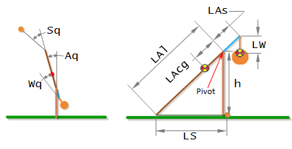
The time derivative of a variable is denoted by appending it with a '. For example Aq' means dAq/dt, and Sq'' means d²Sq/dt².
Additional constants not shown above are:
Grav = Gravitational Acceleration
mA = Mass of Arm
mW = Mass of Weight
mP = Mass of Projectile
IA3 = Inertia of Arm
IW3 = Inertia of Weight
The equations of motion for stage 1 are:
(-mP*LAl^2*(-1+2*SIN(Aq)*COS(Sq)/SIN(Aq+Sq)) + IA3 + IW3 + mA*LAcg^2 +
		mP*LAl^2*SIN(Aq)^2/SIN(Aq+Sq)^2 + mW*(LAs^2+LW^2+2*LAs*LW*COS(Wq)))*
Aq'' + (IW3 + LW*mW*(LW+LAs*COS(Wq)))*Wq''
= Grav*LAcg*mA*SIN(Aq) +
		LAl*LS*mP*(SIN(Sq)*(Aq'+Sq')^2+COS(Sq)*(COS(Aq+Sq)*Sq'*(Sq'+2*Aq')/SIN(Aq+Sq)+(COS(Aq+Sq)/SIN(Aq+Sq)+LAl*COS(Aq)/(LS*SIN(Aq+Sq)))*Aq'^2))
		+
		LAl*mP*SIN(Aq)*(LAl*SIN(Sq)*Aq'^2-LS*(COS(Aq+Sq)*Sq'*(Sq'+2*Aq')/SIN(Aq+Sq)+(COS(Aq+Sq)/SIN(Aq+Sq)+LAl*COS(Aq)/(LS*SIN(Aq+Sq)))*Aq'^2))/SIN(Aq+Sq)
		- Grav*mW*(LAs*SIN(Aq)+LW*SIN(Aq+Wq)) - LAs*LW*mW*SIN(Wq)*(Aq'^2-(Aq'+Wq')^2)
(IW3 + LW*mW*(LW+LAs*COS(Wq)))*Aq''
+ (IW3 + mW*LW^2)*Wq''
= -LW*mW*(Grav*SIN(Aq+Wq)+LAs*SIN(Wq)*Aq'^2)
Note that in stage 1, when the ball is on the ground, the trebuchet only has two degrees of freedom, which is why there are only two equations of motion. However there were three variables to begin with. This works because Sq’ becomes a dependent variable defined by the expression,
Sq'= -(LAl*SIN(Aq)+LS*SIN(Aq+Sq))*Aq'/(LS*SIN(Aq+Sq))
and Sq’’ becomes,
Sq''= -COS(Aq+Sq)*Sq'*(Sq'+2*Aq')/SIN(Aq+Sq) -
(COS(Aq+Sq)/SIN(Aq+Sq)+LAl*COS(Aq)/(LS*SIN(Aq+Sq)))*Aq'^2 -
(LAl*SIN(Aq)+LS*SIN(Aq+Sq))*Aq''/(LS*SIN(Aq+Sq))
As is discussed in the Example Problem, complex differential equations like this are practically impossible to solve analytically. As a result, numerical methods must be used to approximate an answer. These methods require that the equations of motion to be reduced to first order differential equations. In order to accomplish this, we will define three new variables Aw, Ww, and Sw which are the the time derivatives of Aq, Wq, and Sq.
Aw = Aq'
Ww = Wq'
Sw = Sq'
Substituting Aw, Ww, and Sw in to the equations of motion gives,
(-mP*LAl^2*(-1+2*SIN(Aq)*COS(Sq)/SIN(Aq+Sq)) + IA3 + IW3 + mA*LAcg^2 +
		mP*LAl^2*SIN(Aq)^2/SIN(Aq+Sq)^2 + mW*(LAs^2+LW^2+2*LAs*LW*COS(Wq)))*
Aw' + (IW3 + LW*mW*(LW+LAs*COS(Wq)))*Ww'
= Grav*LAcg*mA*SIN(Aq) +
		LAl*LS*mP*(SIN(Sq)*(Aw+Sw)^2+COS(Sq)*(COS(Aq+Sq)*Sw*(Sw+2*Aw)/SIN(Aq+Sq)+(COS(Aq+Sq)/SIN(Aq+Sq)+LAl*COS(Aq)/(LS*SIN(Aq+Sq)))*Aw^2))
		+
		LAl*mP*SIN(Aq)*(LAl*SIN(Sq)*Aw^2-LS*(COS(Aq+Sq)*Sw*(Sw+2*Aw)/SIN(Aq+Sq)+(COS(Aq+Sq)/SIN(Aq+Sq)+LAl*COS(Aq)/(LS*SIN(Aq+Sq)))*Aw^2))/SIN(Aq+Sq)
		- Grav*mW*(LAs*SIN(Aq)+LW*SIN(Aq+Wq)) - LAs*LW*mW*SIN(Wq)*(Aw^2-(Aw+Ww)^2)
(IW3 + LW*mW*(LW+LAs*COS(Wq)))*Aw'
+ (IW3 + mW*LW^2)*Ww'
= -LW*mW*(Grav*SIN(Aq+Wq)+LAs*SIN(Wq)*Aw^2)
which are now first order differntial equations. As discussed in the Example Problem, we need to get the equations into the form,
y'(t) = f(t, y(t))
Separating Aw’ and Ww’ into separate expressions will require a little linear algebra. So, first
we will write the equations of motion in matrix form.
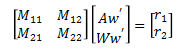
where,
M11= -mP*LAl^2*(-1+2*SIN(Aq)*COS(Sq)/SIN(Aq+Sq)) + IA3 + IW3 + mA*LAcg^2 +
mP*LAl^2*SIN(Aq)^2/SIN(Aq+Sq)^2 + mW*(LAs^2+LW^2+2*LAs*LW*COS(Wq))
M12= IW3 + LW*mW*(LW+LAs*COS(Wq))
M21= IW3 + LW*mW*(LW+LAs*COS(Wq))
M22= IW3 + mW*LW^2
r1= Grav*LAcg*mA*SIN(Aq) +
LAl*LS*mP*(SIN(Sq)*(Aw+Sw)^2+COS(Sq)*(COS(Aq+Sq)*Sw*(Sw+2*Aw)/SIN(Aq+Sq)+(COS(Aq+Sq)/SIN(Aq+Sq)+LAl*COS(Aq)/(LS*SIN(Aq+Sq)))*Aw^2))
+
LAl*mP*SIN(Aq)*(LAl*SIN(Sq)*Aw^2-LS*(COS(Aq+Sq)*Sw*(Sw+2*Aw)/SIN(Aq+Sq)+(COS(Aq+Sq)/SIN(Aq+Sq)+LAl*COS(Aq)/(LS*SIN(Aq+Sq)))*Aw^2))/SIN(Aq+Sq)
- Grav*mW*(LAs*SIN(Aq)+LW*SIN(Aq+Wq)) - LAs*LW*mW*SIN(Wq)*(Aw^2-(Aw+Ww)^2)
r2= -LW*mW*(Grav*SIN(Aq+Wq)+LAs*SIN(Wq)*Aw^2)
We can solve for Aw' and Ww' by multiplying both sides of the equation by the inverse of matrix M.
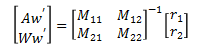
which give the result,
Aw'= (r1*M22-r2*M12)/(M11*M22-M12*M21)
Ww'= -(r1*M21-r2*M11)/(M11*M22-M12*M21)
In summary, the equations that are used by the simulation for stage 1 are,
Aq'= Aw
Wq'= Ww
Sq'= Sw
Aw'= (r1*M22-r2*M12)/(M11*M22-M12*M21)
Ww'= -(r1*M21-r2*M11)/(M11*M22-M12*M21)
Sw'= -COS(Aq+Sq)*Sq'*(Sq'+2*Aq')/SIN(Aq+Sq) -
(COS(Aq+Sq)/SIN(Aq+Sq)+LAl*COS(Aq)/(LS*SIN(Aq+Sq)))*Aq'^2 -
(LAl*SIN(Aq)+LS*SIN(Aq+Sq))*Aq''/(LS*SIN(Aq+Sq))
As described in the Example Problem, these first order differential equations are solved using the numerical methods described in the Runge-Kutta section, and the results are values for the angles (Aq, Wq, Sq) and their derivatives (Aw, Ww, Sw) over time. These angles can be converted into X and Y coordinates using the expressions found in the Angles to XY Coordinates section.
Stage 2:
In stage 2 the parameters are the same as in stage 1. The equations of motion for stage 2 are:
(IA3 + IW3 + mA*LAcg^2 + mP*(LAl^2+LS^2+2*LAl*LS*COS(Sq)) +
		mW*(LAs^2+LW^2+2*LAs*LW*COS(Wq)))*
Aq'' + (IW3 + LW*mW*(LW+LAs*COS(Wq)))*Wq'' + (LS*mP*(LS+LAl*COS(Sq)))*Sq''
= Grav*LAcg*mA*SIN(Aq) + Grav*mP*(LAl*SIN(Aq)+LS*SIN(Aq+Sq)) -
		Grav*mW*(LAs*SIN(Aq)+LW*SIN(Aq+Wq)) - LAl*LS*mP*SIN(Sq)*(Aq'^2-(Aq'+Sq')^2) -
		LAs*LW*mW*SIN(Wq)*(Aq'^2-(Aq'+Wq')^2)
(IW3 + LW*mW*(LW+LAs*COS(Wq)))*Aq''
+ (IW3 + mW*LW^2)*Wq''
= -LW*mW*(Grav*SIN(Aq+Wq)+LAs*SIN(Wq)*Aq'^2)
(LS*mP*(LS+LAl*COS(Sq)))*Aq''
+ (mP*LS^2)*Sq''
= LS*mP*(Grav*SIN(Aq+Sq)-LAl*SIN(Sq)*Aq'^2)
Note that in stage 2, there are three degrees of freedom, so there are now three equations of motion. As in stage 1 we will turn the equations of motion onto first order differential equations by using the time derivatives of Aq, Wq, and Sq, which we will call Aw, Ww, and Sw, and substituting them into the equations of motion.
(IA3 + IW3 + mA*LAcg^2 + mP*(LAl^2+LS^2+2*LAl*LS*COS(Sq)) +
		mW*(LAs^2+LW^2+2*LAs*LW*COS(Wq)))*
Aw' + (IW3 + LW*mW*(LW+LAs*COS(Wq)))*Ww' + (LS*mP*(LS+LAl*COS(Sq)))*Sw'
= Grav*LAcg*mA*SIN(Aq) + Grav*mP*(LAl*SIN(Aq)+LS*SIN(Aq+Sq)) -
		Grav*mW*(LAs*SIN(Aq)+LW*SIN(Aq+Wq)) - LAl*LS*mP*SIN(Sq)*(Aw^2-(Aw+Sw)^2) -
		LAs*LW*mW*SIN(Wq)*(Aw^2-(Aw+Ww)^2)
(IW3 + LW*mW*(LW+LAs*COS(Wq)))*Aw'
+ (IW3 + mW*LW^2)*Ww'
= -LW*mW*(Grav*SIN(Aq+Wq)+LAs*SIN(Wq)*Aw^2)
(LS*mP*(LS+LAl*COS(Sq)))*Aw'
+ (mP*LS^2)*Sw'
= LS*mP*(Grav*SIN(Aq+Sq)-LAl*SIN(Sq)*Aw^2)
In order to separate Aw’, Ww’, and Sw’ into separate expressions we will first put the equations of motion into matrix form.
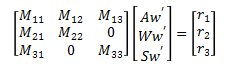
where,
M11= IA3 + IW3 + mA*LAcg^2 + mP*(LAl^2+LS^2+2*LAl*LS*COS(Sq)) +
mW*(LAs^2+LW^2+2*LAs*LW*COS(Wq))
M12= IW3 + LW*mW*(LW+LAs*COS(Wq))
M13= LS*mP*(LS+LAl*COS(Sq))
M21= IW3 + LW*mW*(LW+LAs*COS(Wq))
M22= IW3 + mW*LW^2
M31= LS*mP*(LS+LAl*COS(Sq))
M33= mP*LS^2
r1= Grav*LAcg*mA*SIN(Aq) + Grav*mP*(LAl*SIN(Aq)+LS*SIN(Aq+Sq)) -
Grav*mW*(LAs*SIN(Aq)+LW*SIN(Aq+Wq)) - LAl*LS*mP*SIN(Sq)*(Aw^2-(Aw+Sw)^2) -
LAs*LW*mW*SIN(Wq)*(Aw^2-(Aw+Ww)^2)
r2= -LW*mW*(Grav*SIN(Aq+Wq)+LAs*SIN(Wq)*Aw^2)
r3= LS*mP*(Grav*SIN(Aq+Sq)-LAl*SIN(Sq)*Aw^2)
Now, we can solve for Aw', Ww', and Sw’ by multiplying both sides of the equation by the inverse of matrix M.
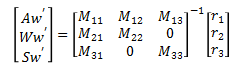
which gives the result used in the simulation,
Aq'= Aw
Wq'= Ww
Sq'= Sw
Aw'= -(r1*M22*M33-r2*M12*M33-r3*M13*M22)/(M13*M22*M31-M33*(M11*M22-M12*M21))
Ww'= (r1*M21*M33-r2*(M11*M33-M13*M31)-r3*M13*M21)/(M13*M22*M31-M33*(M11*M22-M12*M21))
Sw'= (r1*M22*M31-r2*M12*M31-r3*(M11*M22-M12*M21))/(M13*M22*M31-M33*(M11*M22-M12*M21))
As described in the Example Problem, these first order differential equations are solved using the numerical methods described in the Runge-Kutta section, and the results are values for the angles (Aq, Wq, Sq) and their derivatives (Aw, Ww, Sw) over time. These angles can be converted into X and Y coordinates using the expressions found in the Angles to XY Coordinates section.
Stage 3:
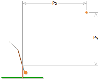
Stage 3 has a different set of parameters than stage 1 or 2. The motion variables are Px and Py. Note that in the simulation everything is measured relative to the pivot point.
The constant parameters in stage 3 are:
Grav = Gravitational Acceleration ρ = Density of Air
WS = Wind Speed
Aeff = Effective Area of the Projectile (= π*(Projectile Diameter/2)^2)
mP = Mass of Projectile
Cd = Drag Coefficient of Projectile
The drag coefficient is not actually a constant. It is related to the Reynolds number which is dependent on the velocity of the projectile relative to the air. For more information on how the drag coefficient is derived, see the Projectile Drag section.
The equations of motion for stage 3 are:
Px''= -(ρ*Cd*Aeff*(Px'-WS)*sqrt(Py'^2+(WS-Px')^2))/(2*mP)
Py''= -Grav - (ρ*Cd*Aeff*Py'*sqrt(Py'^2+(WS-Px')^2))/(2*mP)
In order to make the equations of motion into first order differential equations, we will define to new variables Pvx and Pvy which we will make equal to the time derivatives of Px and Py.
Pvx = Px'
Pvy = Py'
Substituting these into the equations of motion gives the expressions used in the simulation.
Px'= Pvx
Py'= Pvy
Pvx'= -(ρ*Cd*Aeff*(Pvx-WS)*sqrt(Pvy^2+(WS-Pvx)^2))/(2*mP)
Pvy'= -Grav - (ρ*Cd*Aeff*Pvy*sqrt(Pvy^2+(WS-Pvx)^2))/(2*mP)
As described in the Example Problem, these first order differential equations are solved using the numerical methods described in the Runge-Kutta section, and the results are values for the variables (Px, Py) and their derivatives (Pvx, Pvy) over time.