Example Problem
This section does not directly have anything to do with a trebuchet; rather it is an example problem that is used to explain generally the method that I use to make a simulation of a system. If you do not have much experience with simulation, studying this simple example problem will make the trebuchet equations easier to understand.
Developing Equations of Motion
For the example problem we will consider a body in free fall. The first thing we need to do is develop the equations of motion for this system. This is a one-dimensional single body system, so there is only one degree of freedom and thus only one equation of motion.
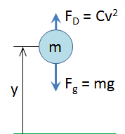
F
g= gravitational forceF
D= force of dragm = mass of the body
g = gravitational constant
C = a constant that depends on the density of the air, the coefficient of drag of the body, and the reference area of the body
v = the velocity of the body
y = height of the body from the ground
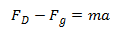
In order to find the equation of motion for this system we will use Newton’s second law: the sum of the forces acting on a body is equal the mass times the acceleration of that body.

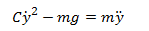
The forces acting on a body in free fall are gravity and the force of drag, so we get,
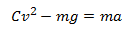
Plugging in the equations for gravity and drag results in,
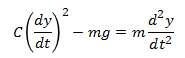
Next we will rewrite the equation in terms of y, where y is the height of the body from the ground. Velocity, v, is the first time-derivative of y, and acceleration, a, is the second time-derivative of y.
I prefer to use dot notation.
We will rewrite this equation in terms of ÿ.
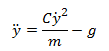
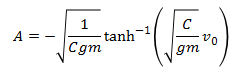
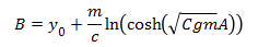
This is the equation of motion for this system. What we really want, however, is an expression for y as a function of time. Since the equation of motion we derived is relatively simple, it is not too difficult to solve it analytically to get y as a function of time. We will not go into the theory behind solving differential equations analytically, but the result of solving our equation of motion for y would be
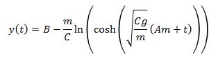
If we were only interested in this problem we could stop here, but we want to solve this problem in a way that is applicable to the trebuchet simulation. It is apparent from this example that the analytical solution for even a simple equation of motion can be fairly complex. For systems with much more complex equations of motion, like the equations of motion for a trebuchet, finding an analytical solution is nearly impossible, so we resort to solving the equation of motion using numerical methods.
Numerical Methods
What we get from a numerical method is different from what we get from an analytical solution. With an analytical solution the result is an expression for the variable(s) of interest as a function of time, and any arbitrary value for time can be plugged into the function to get the value of the variable(s) at that particular time. Using a numerical method will not give us a time function for the variable(s) of interest. With a numerical method we start at a known value for the variable(s), and then calculate what the variable(s) will be after a little bit of time has elapsed. Then we take the new value(s) and calculate what the variable(s) will be after a little more time has elapsed. We keep repeating this to see what the variable(s) do over time. Another thing that is different is that a numerical solution is only an approximation. It can be a very good approximation if it is done right, but it is an approximation none the less, so it is important to evaluate if the error is small enough.
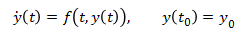
The numerical method we will use for this example is the Euler method. The Euler method assumes you have a function that describes the first derivative of a variable with respect to time, and that you know the initial condition of that variable. The initial condition is what the value of the variable is at time t = 0.
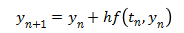
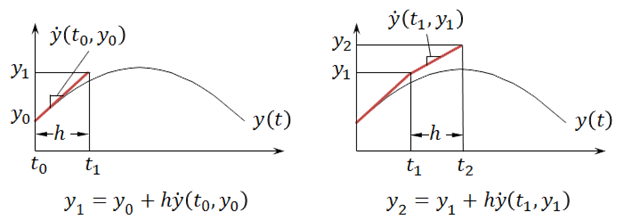
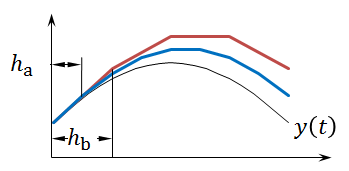
The way the Euler method works is that it takes the current value of y and uses the equation for the time derivative of y to approximate what the value of y will be after some time interval, h.
This equation is easier to visualize with a chart. Note that when using numerical methods y(t) is
not usually known. It is just shown on the chart below for visualization purposes.
Notice the Euler approximation of y does not line up exactly with the actual value of y. This is because the Euler method is just an approximation. If the time interval h is made smaller, then the approximation can be improved. In the chart below the time interval, h, for the blue line is half of that of the red line, and it comes closer to the true curve for y(t).
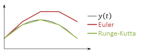
Using a smaller time interval, h, is not the only way to get a more accurate approximation. Another way to get a more accurate result is to use a higher order method. For example, the chart below compares the Euler method to the fourth-order Runge-Kutta method. The same time interval, h, is used for both methods. The fourth-order Runge-Kutta method is much more accurate given the same time interval.
The trebuchet simulation uses the fourth and fifth-order Runge-Kutta methods. However, the higher order methods are more complicated, so for the example problem we will use the Euler method since it is more concise, and the same procedure can be applied to the other methods. The equations for the fourth and fifth-order Runge-Kutta methods are given in the Runge-Kutta section.
Solving the Example Problem Using Numerical Methods
If we want to apply the Euler method to our example problem, we first need to get the equation of motion into the correct form. Remember that the Euler method assumes that we have an expression for the first order derivative of our variable(s) of interest. Our equation of motion, however, is a second order differential equation.
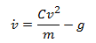
Somehow we need to get first order differential equation(s) from the equation of motion. We will do this by defining a new variable, v (velocity of the body).

If we plug v into our equation of motion we get
Now we have two variables, y and v, and we have expressions for the first order derivative of each variable.

Now we can use the Euler method to solve these equations numerically. Using the Euler method does not give us a general solution to the equations. It is used to find the solution for a particular case, so to continue the example we have to assign values to all the system parameters, and solve the problem for that specific case. We will use the following values for the system parameters.
g (gravitational constant) = 9.8 m/s² (in the negative y direction)
m (mass of body) = 1 kg
C (drag constant) = 0.015 kg/m
y₀ (initial height of body) = 10 m
v₀ (initial velocity of body) = 3 m/s (in the positive y direction)
h (time interval) = 0.1 s
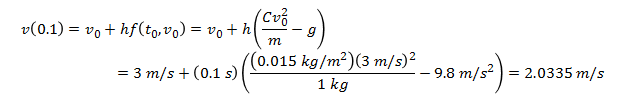
Now that we have given values to all the parameters, we can use the Euler method to find the position of the body after 0.1 seconds.

Now we have the approximate values for the height of the ball and the velocity of the ball after 0.1 seconds, and we can use that result to find the values after 0.2 seconds.


We can repeat this process for as much time as we are interested in. For this example we will follow the body until it reaches the ground. To be concise, we will not show the full equations for every step, rather the results will be summarized in the following table.
| Step | t (s) | y (m) | v (m/s) |
|---|---|---|---|
| 0 | 0.0 | 10.0000 | 3.0000 |
| 1 | 0.1 | 10.3000 | 2.0335 |
| 2 | 0.2 | 10.5034 | 1.0597 |
| 3 | 0.3 | 10.6093 | 0.0814 |
| 4 | 0.4 | 10.6175 | -0.8986 |
| 5 | 0.5 | 10.5276 | -1.8774 |
| 6 | 0.6 | 10.3399 | -2.8521 |
| 7 | 0.7 | 10.0546 | -3.8199 |
| 8 | 0.8 | 9.6727 | -4.7780 |
| 9 | 0.9 | 9.1949 | -5.7238 |
| 10 | 1.0 | 8.6225 | -6.6546 |
| 11 | 1.1 | 7.9570 | -7.5682 |
| 12 | 1.2 | 7.2002 | -8.4623 |
| 13 | 1.3 | 6.3540 | -9.3349 |
| 14 | 1.4 | 5.4205 | -10.1842 |
| 15 | 1.5 | 4.4021 | -11.0086 |
| 16 | 1.6 | 3.3012 | -11.8068 |
| 17 | 1.7 | 2.1205 | -12.5777 |
| 18 | 1.8 | 0.8628 | -13.3204 |
| 19 | 1.9 | -0.4693 | -14.0343 |
We can see that at step 19 the value for y went negative which means the body hit the ground sometime between 1.8 and 1.9 seconds. The results of this problem summarized in the table are plotted in the graph below.
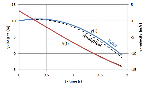
As mentioned before this is only an approximation of the results. Since we also have the analytical solution to this problem we can compare the results that we got from using the Euler method to the exact values from the analytical solution. The dotted line shows the analytical solution.
This simple example should have demonstrated the essentials of what is needed to understand what is going on in the trebuchet simulation. First the equations of motion are derived. They are then then reduced to first order differential equations and then solved using a numerical method like the Euler or Runge-Kutta method.
This example problem should have helped prepared you for the Equations of Motion and Runge-Kutta sections.