Autolev
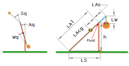
The equations of motion for the trebuchet were derived using a program called Autolev. The Autolev code that was used to derive the trebuchet equations will be included here with some minimal explanation. The figure below shows what the constants and variables in this code correspond to.
Stage 1 Autolev Code:
(1) % File: Trebuchet_Stage_1.al
(2) % Date: November 19, 2010
(3) % Author: Eric Olson
(4) % Problem: This is the first stage in a simulation of a trebuchet
(5) % shooting a projectile. In this stage the projectile
(6) % is in the sling, and is in contact with the ground.
(7) %--------------------------------------------------------------------
(8) % Default settings
Anything after a % symbol is just a comment.
(9) AutoEpsilon 1.0E-14 % Rounds off to nearest integer
(10) AutoZ OFF % Turn ON for large problems
(11) Digits 7 % Number of digits displayed for numbers
(12) BeepSound OFF
These are just program settings that can be ignored.
(13) %--------------------------------------------------------------------
(14) % Newtonian, bodies, frames, particles, points
(15) Newtonian N % Newtonian reference frame
The Newtonian reference frame is the base reference frame that everything else is based off of.
(16) Bodies A, W % Arm and Counterweight
A body has a local reference frame, a mass, a center of gravity, and inertia properties.
(17) Frames S % Sling
The sling is assumed to be massless, so it is defined as a frame instead of as a body.
(18) Particles P % Projectile
The projectile is assumed to be a point mass.
(19) %--------------------------------------------------------------------
(20) % Variables, constants, and specified
(21) Variables Aq', Wq', Sq' % Arm angle, Counterweight-arm angle, and Sling-arm
		angle
This defined the angles and their derivatives. The angles are the “motion variables”.
(22) Variables Fy % Normal Force of Projectile
This is the force that the ground exerts on the projectile in stage 1.
(23) Constants Grav % Local gravitational acceleration
(24) Constants LAs, LAl, LAcg % Length of long arm, length of short arm, distance from pivot to
		Arm CG.
(25) Constants LW, LS, h % Distance from arm end to Wo, length of sling, hight of pivot from
		the ground
(26) %--------------------------------------------------------------------
(27) % Motion variables for static/dynamic analysis
(28) Variables u3' % Motion variables; derivatives
(29) Aq' = u1
-> (30) Aq' = u1
The -> means that this line is program output.
(31) Wq' = u2
-> (32) Wq' = u2
(33) Sq' = u3
-> (34) Sq' = u3
This section defines the derivatives of the motion variables. This is done this way so that the equations for the trebuchet will be first order differential equations rather that second order differential equations. The numerical methods that are used to solve the final equations only work with first order differential equations. This is similar to what we did in the Example Problem.
(35) %--------------------------------------------------------------------
(36) % Quantities to be left explicit
(37) Zee_Not = [u1',u2',u3',Grav]
-> (38) Zee_Not = [u1', u2', u3', Grav]
With the initial settings that were set, this section does not do anything.
(39) %--------------------------------------------------------------------
(40) % Mass and inertia properties
(41) Mass A=mA, W=mW, P=mP
(42) Inertia A, IA1, IA2, IA3
-> (43) I_A_AO>> = IA1*A1>*A1> + IA2*A2>*A2> + IA3*A3>*A3>
(44) Inertia W, IW1, IW2, IW3
-> (45) I_W_WO>> = IW1*W1>*W1> + IW2*W2>*W2> + IW3*W3>*W3>
This section assigns mass and inertia to the bodies. The convention in Autolev is that 1 is x, 2 is y, and 3 is z. Anything with a > symbol is a vector, and anything with a >> is a tensor. A1> means the x direction of the local reference frame associated with body A.
(46) %--------------------------------------------------------------------
(47) % Geometry relating unit vectors
(48) Simprot(N, A, 3, Aq)
-> (49) N_A = [COS(Aq), -SIN(Aq), 0; SIN(Aq), COS(Aq), 0; 0, 0, 1]
(50) Simprot(A, W, 3, Wq)
-> (51) A_W = [COS(Wq), -SIN(Wq), 0; SIN(Wq), COS(Wq), 0; 0, 0, 1]
(52) Simprot(A, S, 3, Sq)
-> (53) A_S = [COS(Sq), -SIN(Sq), 0; SIN(Sq), COS(Sq), 0; 0, 0, 1]
This section defines the relationship between the different local reference frames and the Newtonian reference frame.
(54) %--------------------------------------------------------------------
(55) % Angular velocities
(56) W_A_N> = Aq'*N3>
-> (57) W_A_N> = u1*A3>
(58) W_W_A> = Wq'*A3>
-> (59) W_W_A> = u2*A3>
(60) W_S_A> = Sq'*A3>
-> (61) W_S_A> = u3*A3>
(62) %--------------------------------------------------------------------
(63) % Position vectors
(64) P_No_Ao> = LAcg*A2>
-> (65) P_No_Ao> = LAcg*A2>
(66) P_No_Wo> = -LAs*A2> - LW*W2>
-> (67) P_No_Wo> = -LAs*A2> - LW*W2>
(68) P_No_P> = LAl*A2> + LS*S2>
-> (69) P_No_P> = LAl*A2> + LS*S2>
This section defines the location of the different points of interest in the trebuchet. For example line 66 says the vector from the pivot (No) to the CG of the weight (Wo) is –LAs in the y component of the arm’s local coordinate system, and –LW in the y component of the weight’s local coordinate system.
(70) %--------------------------------------------------------------------
(71) % Velocities
(72) V_Ao_N> = Dt(P_No_Ao>,N)
-> (73) V_Ao_N> = -LAcg*u1*A1>
(74) V_Wo_N> = Dt(P_No_Wo>,N)
-> (75) V_Wo_N> = LAs*u1*A1> + LW*(u1+u2)*W1>
(76) V_P_N> = Dt(P_No_P>,N)
-> (77) V_P_N> = -LAl*u1*A1> - LS*(u1+u3)*S1>
The velocities vectors of the points of interest are defined as the time derivatives of the position vectors in reference to the Newtonian reference frame.
(78) Projectile_Vx = coef(express(V_P_N>,N),N1>)
-> (79) Projectile_Vx = -LAl*COS(Aq)*u1 - LS*COS(Aq+Sq)*(u1+u3)
(80) Projectile_Vy = coef(express(V_P_N>,N),N2>)
-> (81) Projectile_Vy = -LAl*SIN(Aq)*u1 - LS*SIN(Aq+Sq)*(u1+u3)
This finds the x and y component of the projectile velocity expressed in terms of the Newtonian reference frame.
(82) %--------------------------------------------------------------------
(83) % Motion constraints
(84) Auxiliary[1] = Projectile_Vy % P stays on ground
-> (85) Auxiliary[1] = Projectile_Vy
(86) Constrain(Auxiliary[u3])
-> (87) u3 = -(LAl*SIN(Aq)+LS*SIN(Aq+Sq))*u1/(LS*SIN(Aq+Sq))
-> (88) u3' = -COS(Aq+Sq)*u3*(u3+2*u1)/SIN(Aq+Sq) - (COS(Aq+Sq)/SIN(Aq+Sq)+LAl*
COS(Aq)/(LS*SIN(Aq+Sq)))*u1^2-(LAl*SIN(Aq)+LS*SIN(Aq+Sq))*u1'/(LS*SIN
(Aq+Sq))
This section constrains the y component of the projectiles velocity to be 0. This is what keeps the projectile moving along the ground in the first stage. This constraint eliminates one degree of freedom from the system and so one of the motion variables has to be rewritten in terms of the other motion variables. In this case u3 aka Sq’ is now given in terms of u1 and u2, and will not show up in the final equations.
(89) %Dependent[1] = Projectile_Vy % P stays on ground
(90) %Constrain(Dependent[u3])
(91) %--------------------------------------------------------------------
(92) % Angular accelerations
(93) ALF_A_N> = Dt(W_A_N>,N)
-> (94) ALF_A_N> = u1'*A3>
(95) ALF_W_N> = Dt(W_W_N>,N)
-> (96) ALF_W_N> = (u1'+u2')*W3>
(97) ALF_S_N> = Dt(W_S_N>,N)
-> (98) ALF_S_N> = (u1'+u3')*A3>
The angular accelerations are found by taking the time derivatives of the angular velocities.
(99) %--------------------------------------------------------------------
(100) % Accelerations
(101) A_Ao_N> = Dt(V_Ao_N>,N)
-> (102) A_Ao_N> = -LAcg*u1'*A1> - LAcg*u1^2*A2>
(103) A_Wo_N> = Dt(V_Wo_N>,N)
-> (104) A_Wo_N> = LAs*u1'*A1> + LAs*u1^2*A2> + LW*(u1'+u2')*W1> +
		LW*(u1+u2)^2
*W2>
(105) A_P_N> = Dt(V_P_N>,N)
-> (106) A_P_N> = -LAl*u1'*A1> - LAl*u1^2*A2> - LS*(u1'+u3')*S1> -
		LS*(u1+u3)^2
*S2>
The acceleration vectors of the points of interest are found by taking the derivative of the velocity vectors.
(107) %--------------------------------------------------------------------
(108) % Forces
(109) Force_P> = Fy*N2>
-> (110) Force_P> = Fy*N2>
This defines the force vector exerted on the projectile by the ground.
(111) Gravity(-Grav*N2>)
-> (112) FORCE_AO> = -Grav*mA*N2>
-> (113) FORCE_P> = (Fy-Grav*mP)*N2>
-> (114) FORCE_WO> = -Grav*mW*N2>
This defines the force vectors that gravity exerts on the bodies and point masses.
(115) %--------------------------------------------------------------------
(116) % Equations of motion
(117) Zero = Fr() + FrStar() % Find equations of motion
-> (118) Zero[1] = Grav*LAcg*mA*SIN(Aq) + (Grav*mP-Fy)*(LAl*SIN(Aq)+LS*SIN(Aq+
Sq)) - Grav*mW*(LAs*SIN(Aq)+LW*SIN(Aq+Wq)) - LAs*LW*mW*SIN(Wq)*(u1^2-(
u1+u2)^2) - LS*mP*(LAl*SIN(Sq)*u1^2-LAl*SIN(Sq)*(u1+u3)^2-LS*(COS(Aq+
Sq)*u3*(u3+2*u1)/SIN(Aq+Sq)+(COS(Aq+Sq)/SIN(Aq+Sq)+LAl*COS(Aq)/(LS*SIN
(Aq+Sq)))*u1^2)-LAl*COS(Sq)*(COS(Aq+Sq)*u3*(u3+2*u1)/SIN(Aq+Sq)+(COS(
Aq+Sq)/SIN(Aq+Sq)+LAl*COS(Aq)/(LS*SIN(Aq+Sq)))*u1^2)) - (IW3+LW*mW*(
LW+LAs*COS(Wq)))*u2' - (IA3+IW3+mA*LAcg^2+mW*(LAs^2+LW^2+2*LAs*LW*COS(
Wq))-mP*(LAl^2*SIN(Aq)*COS(Sq)/SIN(Aq+Sq)-LAl^2-LAl*LS*COS(Sq)-LS^2*(1
-(LAl*SIN(Aq)+LS*SIN(Aq+Sq))/(LS*SIN(Aq+Sq)))))*u1'
-> (119) Zero[2] = -Grav*LW*mW*SIN(Aq+Wq) - LAs*LW*mW*SIN(Wq)*u1^2 - (IW3+mW*
LW^2)*u2' - (IW3+LW*mW*(LW+LAs*COS(Wq)))*u1'
-> (120) Zero[3] = LS*(SIN(Aq+Sq)*(Grav*mP-Fy)+mP*(LS*(COS(Aq+Sq)*u3*(u3+2*u1)/
SIN(Aq+Sq)+(COS(Aq+Sq)/SIN(Aq+Sq)+LAl*COS(Aq)/(LS*SIN(Aq+Sq)))*u1^2)-
LAl*SIN(Sq)*u1^2-LAl*(COS(Sq)-SIN(Aq)/SIN(Aq+Sq))*u1'))
The trebuchet has been fully defined by all the previous sections. This section combines it all into the equations of motion of the trebuchet in stage 1. Notice that there are tree equations of motion but only two motion variables derivatives appear in these equations (u1 and u2). This is because u3 was turned into a dependent variable in line (86).
(121) Kane(Fy)
-> (122) Fy = mP*(Grav+(LS*(COS(Aq+Sq)*u3*(u3+2*u1)/SIN(Aq+Sq)+(COS(Aq+Sq)/SIN(
Aq+Sq)+LAl*COS(Aq)/(LS*SIN(Aq+Sq)))*u1^2)-LAl*SIN(Sq)*u1^2-LAl*(COS(
Sq)-SIN(Aq)/SIN(Aq+Sq))*u1')/SIN(Aq+Sq))
-> (123) ZERO[1] = Grav*LAcg*mA*SIN(Aq) + LAl*LS*mP*(SIN(Sq)*(u1+u3)^2+COS(Sq)*
(COS(Aq+Sq)*u3*(u3+2*u1)/SIN(Aq+Sq)+(COS(Aq+Sq)/SIN(Aq+Sq)+LAl*COS(Aq)
/(LS*SIN(Aq+Sq)))*u1^2)) + LAl*mP*SIN(Aq)*(LAl*SIN(Sq)*u1^2-LS*(COS(
Aq+Sq)*u3*(u3+2*u1)/SIN(Aq+Sq)+(COS(Aq+Sq)/SIN(Aq+Sq)+LAl*COS(Aq)/(LS*
SIN(Aq+Sq)))*u1^2))/SIN(Aq+Sq) - Grav*mW*(LAs*SIN(Aq)+LW*SIN(Aq+Wq))
- LAs*LW*mW*SIN(Wq)*(u1^2-(u1+u2)^2) - (IW3+LW*mW*(LW+LAs*COS(Wq)))*
u2' - (IA3+IW3+mA*LAcg^2+mP*LAl^2+mW*(LAs^2+LW^2+2*LAs*LW*COS(Wq))-mP*
LAl^2*SIN(Aq)*(2*COS(Sq)-SIN(Aq)/SIN(Aq+Sq))/SIN(Aq+Sq))*u1'
-> (124) ZERO[2] = -LW*mW*(Grav*SIN(Aq+Wq)+LAs*SIN(Wq)*u1^2) - (IW3+mW*LW^2)*
u2' - (IW3+LW*mW*(LW+LAs*COS(Wq)))*u1'
Fy was defined as the force to keep the projectile on the ground. This command converted the previous three equations of motion into the two equations of motion that are expected, and an expression for Fy. This is where the equations of motion for stage 1 of the Equations of Motion section came from.
Stage 2 Autolev Code:
The stage 2 Autolev code is very similar to the stage 1 code, so only the parts that are different will be explained.
(1) % File: Trebuchet_Stage_2.al
(2) % Date: November 5, 2010
(3) % Author: Eric Olson
(4) % Problem: This is the second stage in a simulation of a trebuchet
(5) % shooting a projectile. In this stage the projectile
(6) % is in the sling, and is not in contact with the ground.
(7) %--------------------------------------------------------------------
(8) % Default settings
(9) AutoEpsilon 1.0E-14 % Rounds off to nearest integer
(10) AutoZ OFF % Turn ON for large problems
(11) Digits 7 % Number of digits displayed for numbers
(12) BeepSound OFF
(13) %--------------------------------------------------------------------
(14) % Newtonian, bodies, frames, particles, points
(15) Newtonian N % Newtonian referance frame
(16) Bodies A, W % Arm and Counterweight
(17) Frames S % Sling
(18) Particles P % Projectile
(19) %--------------------------------------------------------------------
(20) % Variables, constants, and specified
(21) Variables Aq', Wq', Sq' % Arm angle, Counterweight-arm angle, and Sling-arm
		angle
(22) Constants Grav % Local gravitational acceleration
(23) Constants LAs, LAl, LAcg % Length of long arm, length of short arm, distance from pivot to
		Arm CG.
(24) Constants LW, LS, h % Distance from arm end to Wo, length of sling, hight of pivot from
		the ground
(25) %--------------------------------------------------------------------
(26) % Motion variables for static/dynamic analysis
(27) Variables u3' % Motion variables; derivatives
(28) Aq' = u1
-> (29) Aq' = u1
(30) Wq' = u2
-> (31) Wq' = u2
(32) Sq' = u3
-> (33) Sq' = u3
(34) %--------------------------------------------------------------------
(35) % Quantities to be left explicit
(36) Zee_Not = [u1',u2',u3',Grav]
-> (37) Zee_Not = [u1', u2', u3', Grav]
(38) %--------------------------------------------------------------------
(39) % Mass and inertia properties
(40) Mass A=mA, W=mW, P=mP
(41) Inertia A, IA1, IA2, IA3
-> (42) I_A_AO>> = IA1*A1>*A1> + IA2*A2>*A2> + IA3*A3>*A3>
(43) Inertia W, IW1, IW2, IW3
-> (44) I_W_WO>> = IW1*W1>*W1> + IW2*W2>*W2> + IW3*W3>*W3>
(45) %--------------------------------------------------------------------
(46) % Geometry relating unit vectors
(47) Simprot(N, A, 3, Aq)
-> (48) N_A = [COS(Aq), -SIN(Aq), 0; SIN(Aq), COS(Aq), 0; 0, 0, 1]
(49) Simprot(A, W, 3, Wq)
-> (50) A_W = [COS(Wq), -SIN(Wq), 0; SIN(Wq), COS(Wq), 0; 0, 0, 1]
(51) Simprot(A, S, 3, Sq)
-> (52) A_S = [COS(Sq), -SIN(Sq), 0; SIN(Sq), COS(Sq), 0; 0, 0, 1]
(53) %--------------------------------------------------------------------
(54) % Angular velocities
(55) W_A_N> = Aq'*N3>
-> (56) W_A_N> = u1*A3>
(57) W_W_A> = Wq'*A3>
-> (58) W_W_A> = u2*A3>
(59) W_S_A> = Sq'*A3>
-> (60) W_S_A> = u3*A3>
(61) %--------------------------------------------------------------------
(62) % Position vectors
(63) P_No_Ao> = LAcg*A2>
-> (64) P_No_Ao> = LAcg*A2>
(65) P_No_Wo> = -LAs*A2> - LW*W2>
-> (66) P_No_Wo> = -LAs*A2> - LW*W2>
(67) P_No_P> = LAl*A2> + LS*S2>
-> (68) P_No_P> = LAl*A2> + LS*S2>
(69) %--------------------------------------------------------------------
(70) % Velocities
(71) V_Ao_N> = Dt(P_No_Ao>,N)
-> (72) V_Ao_N> = -LAcg*u1*A1>
(73) V_Wo_N> = Dt(P_No_Wo>,N)
-> (74) V_Wo_N> = LAs*u1*A1> + LW*(u1+u2)*W1>
(75) V_P_N> = Dt(P_No_P>,N)
-> (76) V_P_N> = -LAl*u1*A1> - LS*(u1+u3)*S1>
(77) %--------------------------------------------------------------------
(78) % Angular accelerations
(79) ALF_A_N> = Dt(W_A_N>,N)
-> (80) ALF_A_N> = u1'*A3>
(81) ALF_W_N> = Dt(W_W_N>,N)
-> (82) ALF_W_N> = (u1'+u2')*W3>
(83) ALF_S_N> = Dt(W_S_N>,N)
-> (84) ALF_S_N> = (u1'+u3')*A3>
(85) %--------------------------------------------------------------------
(86) % Accelerations
(87) A_Ao_N> = Dt(V_Ao_N>,N)
-> (88) A_Ao_N> = -LAcg*u1'*A1> - LAcg*u1^2*A2>
(89) A_Wo_N> = Dt(V_Wo_N>,N)
-> (90) A_Wo_N> = LAs*u1'*A1> + LAs*u1^2*A2> + LW*(u1'+u2')*W1> +
		LW*(u1+u2)^2*
W2>
(91) A_P_N> = Dt(V_P_N>,N)
-> (92) A_P_N> = -LAl*u1'*A1> - LAl*u1^2*A2> - LS*(u1'+u3')*S1> -
		LS*(u1+u3)^2*
S2>
(93) %--------------------------------------------------------------------
(94) % Forces
(95) Gravity(-Grav*N2>)
-> (96) FORCE_AO> = -Grav*mA*N2>
-> (97) FORCE_P> = -Grav*mP*N2>
-> (98) FORCE_WO> = -Grav*mW*N2>
(99) %--------------------------------------------------------------------
(100) % Equations of motion
(101) Zero = Fr() + FrStar() % Find equations of motion
-> (102) Zero[1] = Grav*LAcg*mA*SIN(Aq) + Grav*mP*(LAl*SIN(Aq)+LS*SIN(Aq+Sq))
- Grav*mW*(LAs*SIN(Aq)+LW*SIN(Aq+Wq)) - LAl*LS*mP*SIN(Sq)*(u1^2-(u1+
u3)^2) - LAs*LW*mW*SIN(Wq)*(u1^2-(u1+u2)^2) - LS*mP*(LS+LAl*COS(Sq))*
u3' - (IW3+LW*mW*(LW+LAs*COS(Wq)))*u2' - (IA3+IW3+mA*LAcg^2+mP*(LAl^2+
LS^2+2*LAl*LS*COS(Sq))+mW*(LAs^2+LW^2+2*LAs*LW*COS(Wq)))*u1'
-> (103) Zero[2] = -Grav*LW*mW*SIN(Aq+Wq) - LAs*LW*mW*SIN(Wq)*u1^2 - (IW3+mW*
LW^2)*u2' - (IW3+LW*mW*(LW+LAs*COS(Wq)))*u1'
-> (104) Zero[3] = LS*mP*(Grav*SIN(Aq+Sq)-LAl*SIN(Sq)*u1^2-LS*u3'-(LS+LAl*COS(
Sq))*u1')
Notice that in stage 2 there are no dependent variables, so u1’, u2’, and u3’ all appear, and there are three equations and three motion variable derivatives. This is where the equations of motion for stage 2 of the Equations of Motion section came from.
Stage 3 Autolev Code:
Sage 3 was originally solved with the trebuchet still moving after the projectile had been released, however to speed up computation time only the projectile portions of the equations were used, so only the parts of the stage 3 Autolev file that have to do with the projectile will be shown.
(1) % File: Trebuchet_Stage_3_With_Drag_and_Wind_Speed.al
(2) % Date: March 10, 2013
(3) % Author: Eric Olson
(4) % Problem: This is the last stage in a simulation of a trebuchet
(5) % shooting a projectile. In this stage the projectile
(6) % has left the sling.
(7) % This version includes drag and wind speed.
(8) %--------------------------------------------------------------------
(9) % Default settings
(10) AutoEpsilon 1.0E-14 % Rounds off to nearest integer
(11) AutoZ OFF % Turn ON for large problems
(12) Digits 7 % Number of digits displayed for numbers
(13) BeepSound OFF
(14) %--------------------------------------------------------------------
(15) % Newtonian, bodies, frames, particles, points
(16) Newtonian N % Newtonian referance frame
(17) Bodies A, W % Arm and Counterweight
(18) Frames S % Sling
(19) Particles P % Projectile
(20) %--------------------------------------------------------------------
(21) % Variables, constants, and specified
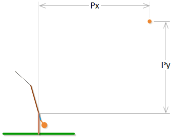
(22) Variables Aq',Wq',Px',Py' % Arm angle, Counterweight-arm angle, and
		Sling-arm angle
Px and Py are the x and y coordinates of the projectile. In the stage 3 they are motion variables.
(23) Constants Grav % Local gravitational acceleration
(26) %--------------------------------------------------------------------
(27) % Motion variables for static/dynamic analysis
(28) Variables u4' % Motion variables; derivatives
(33) Px' = u3
-> (34) Px' = u3
(35) Py' = u4
-> (36) Py' = u4
(37) %--------------------------------------------------------------------
(38) % Quantities to be left explicit
(39) Zee_Not = [u1',u2',u3',u4',Grav]
-> (40) Zee_Not = [u1', u2', u3', u4', Grav]
(41) %--------------------------------------------------------------------
(42) % Mass and inertia properties
(43) Mass A=mA, W=mW, P=mP
(60) %--------------------------------------------------------------------
(61) % Position vectors
(66) P_No_P> = Px*N1> + Py*N2>
-> (67) P_No_P> = Px*N1> + Py*N2>
(68) %--------------------------------------------------------------------
(69) % Velocities
(74) V_P_N> = Dt(P_No_P>,N)
-> (75) V_P_N> = u3*N1> + u4*N2>
(82) %--------------------------------------------------------------------
(83) % Accelerations
(88) A_P_N> = Dt(V_P_N>,N)
-> (89) A_P_N> = u3'*N1> + u4'*N2>
(90) %--------------------------------------------------------------------
(91) % Forces
(92) constant AirDensity, EffectiveArea, Cd
(93) constant WindSpeed
(94) Force_P> = -0.5*AirDensity*EffectiveArea*Cd*Dot(V_P_N> - WindSpeed*N1>,
V_P_N> - WindSpeed*N1>)*(V_P_N> - WindSpeed*N1>)/mag(V_P_N> -
WindSpeed*N1>)
-> (95) Force_P> = 0.5*AirDensity*Cd*EffectiveArea*(WindSpeed-u3)*(u4^2+(WindS
peed-u3)^2)^0.5*N1> - 0.5*AirDensity*Cd*EffectiveArea*u4*(u4^2+(WindSp
eed-u3)^2)^0.5*N2>
(96) Gravity(-Grav*N2>)
-> (98) FORCE_P> = 0.5*AirDensity*Cd*EffectiveArea*(WindSpeed-u3)*(u4^2+(WindS
peed-u3)^2)^0.5*N1> + (-Grav*mP-0.5*AirDensity*Cd*EffectiveArea*u4*(u4^
2+(WindSpeed-u3)^2)^0.5)*N2>
(100) %--------------------------------------------------------------------
(101) % Equations of motion
(102) Zero = Fr() + FrStar() % Find equations of motion
-> (105) Zero[3] = 0.5*AirDensity*Cd*EffectiveArea*(WindSpeed-u3)*(u4^2+(WindS
peed-u3)^2)^0.5 - mP*u3'
-> (106) Zero[4] = -Grav*mP - 0.5*AirDensity*Cd*EffectiveArea*u4*(u4^2+(WindSp
eed-u3)^2)^0.5 - mP*u4'
This is where the equations of motion for stage 3 of the Equations of Motion section came from.